Download
1 / 39
410 likes | 596 Views
Correlation and Regression. Quantitative Methods in HPELS 440:210. Agenda. Introduction The Pearson Correlation Hypothesis Tests with the Pearson Correlation Regression Instat Nonparametric versions. Introduction.

E N D
Correlation and Regression Quantitative Methods in HPELS 440:210
Agenda • Introduction • The Pearson Correlation • Hypothesis Tests with the Pearson Correlation • Regression • Instat • Nonparametric versions
Introduction • Correlation: Statistical technique used to measure and describe a relationship between two variables • Direction of relationship: • Positive • Negative • Form of relationship: • Linear • Quadratic . . . • Degree of relationship: • -1.0 0.0 +1.0
Uses of Correlations • Prediction • Validity • Reliability
Agenda • Introduction • The Pearson Correlation • Hypothesis Tests with the Pearson Correlation • Regression • Instat • Nonparametric versions
The Pearson Correlation • Statistical Notation Recall for ANOVA: • r = Pearson correlation • SP = sum of products of deviations • Mx = mean of x scores • SSx = sum of squares of x scores
Pearson Correlation • Formula Considerations Recall for ANOVA: • SP = S(X – Mx)(Y – My) • SP = SXY – SXSY / n • SSx = S(X – Mx)2 • SSy = S(Y – My)2 • r = SP / √SSxSSy
Pearson Correlation • Step 1: Calculate SP • Step 2: Calculate SS for X and Y values • Step 3: Calcuate r
Step 1 SP SXY = (0*1)+(10*3)+(4*1)+(8*2)+(8*3) SXY = 0 + 30 + 4 + 16 + 24 SXY = 74 SP = SXY – SXSY / n SP = 74 – [30(100)]/5 SP = 74 - 60 SP = 14 SP = S(X – Mx)(Y – My) SP = (-6*-1)+(4*1)+(-2*-1)+(2*0)+(2*1) SP = 6 + 4 + 2 + 0 + 2 SP = 14 SX=30 SY=10
Step 3 r • r = SP / √SSxSSy • r = 14 / √(64)(4) • r = 14 / √256 • r = 14/16 • r = 0.875
Interpretation of r • Correlation ≠ causality • Restricted range • If data does not represent the full range of scores – be wary • Outliers can have a dramatic effect • Figure 16.9 • Correlation and variability • Coefficient of determination (r2)
Agenda • Introduction • The Pearson Correlation • Hypothesis Tests with the Pearson Correlation • Regression • Instat • Nonparametric versions
The Process • Step 1: State hypotheses • Non directional: • H0: ρ = 0 (no population correlation) • H1: ρ ≠ 0 (population correlation exists) • Directional: • H0: ρ ≤ 0 (no positive population correlation) • H1: ρ < 0 (positive population correlation exists) • Step 2: Set criteria • a = 0.05 • Step 3: Collect data and calculate statistic • r • Step 4: Make decision • Accept or reject
Example • Researchers are interested in determining if leg strength is related to jumping ability • Researchers measure leg strength with 1RM squat (lbs) and vertical jump height (inches) in 5 subjects (n = 5)
Step 1: State Hypotheses Non-Directional H0: ρ = 0 H1: ρ ≠ 0 Critical value = 0.878 Step 2: Set Criteria Alpha (a) = 0.05 Critical Value: Use Critical Values for Pearson Correlation Table Appendix B.6 (p 697) 0.878 Information Needed: df = n - 2 Alpha (a) = 0.05 Directional or non-directional?
Step 3: Collect Data and Calculate Statistic Data: Calculate SP SP = SXY – SXSY / n SP = 27135 – [1065(126)]/5 SP = 27135 - 26838 SP = 297 Calculate SSx S M S
Step 3: Collect Data and Calculate Statistic Calculate SSy M S M S Step 4: Make Decision 0.667 < 0.878 Accept or reject? Calculate r r = SP / √SSxSSy r = 297 / √11780(16.8) r = 297 / √197904 r = 297 / 444.86 r = 0.667
Agenda • Introduction • The Pearson Correlation • Hypothesis Tests with the Pearson Correlation • Regression • Instat • Nonparametric versions
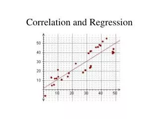
Regression • Recall Several uses of correlation: • Prediction • Validity • Reliability • Regression attempts to predict one variable based on information about the other variable • Line of best fit
Regression • Line of best fit can be described with the following linear equation Y = bX + a where: • Y = predicted Y value • b = slope of line • X = any X value • a = intercept
25 5 Y = bX + a, where: Y = cost (?) b = cost per hour ($5) X = number of hours (?) a = membership cost ($25) Y = 5X + 25 Y = 5(10) + 25 Y = 50 + 25 = 75 Y = 5X + 25 Y = 5(30) + 25 Y = 150 + 25 = 175
Calculation of the Regression Line • Regression line = line of best fit = linear equation • SP = S(X – Mx)(Y – My) • SSx = S(X – Mx)2 • b = SP / SSx • a = My - bMx
Example 16.14, p 557 Mx=5 My=6 SP = S(X – Mx)(Y – My) SP = 16 SSx = S(X – Mx)2 SP = 10 b = SP / SSx b = 16 / 10 = 1.6 a = My - bMx a = 6 – 1.6(5) = -2 Y = bX + a Y = 1.6(X) - 2
Agenda • Introduction • The Pearson Correlation • Hypothesis Tests with the Pearson Correlation • Regression • Instat • Nonparametric versions
Instat - Correlation • Type data from sample into a column. • Label column appropriately. • Choose “Manage” • Choose “Column Properties” • Choose “Name” • Choose “Statistics” • Choose “Regression” • Choose “Correlation”
Instat – Correlation • Choose the appropriate variables to be correlated • Click OK • Interpret the p-value
Instat – Regression • Type data from sample into a column. • Label column appropriately. • Choose “Manage” • Choose “Column Properties” • Choose “Name” • Choose “Statistics” • Choose “Regression” • Choose “Simple”
Instat – Regression • Choose appropriate variables for: • Response (Y) • Explanatory (X) • Check “significance test” • Check “ANOVA table” • Check “Plots” • Click OK • Interpret p-value
Reporting Correlation Results • Information to include: • Value of the r statistic • Sample size • p-value • Examples: • A correlation of the data revealed that strength and jumping ability were not significantly related (r = 0.667, n = 5, p > 0.05) • Correlation matrices are used when interrelationships of several variables are tested (Table 1, p 541)
Agenda • Introduction • The Pearson Correlation • Hypothesis Tests with the Pearson Correlation • Regression • Instat • Nonparametric versions
Nonparametric Versions • Spearman rho when at least one of the data sets is ordinal • Point biserial correlation when one set of data is ratio/interval and the other is dichotomous • Male vs. female • Success vs. failure • Phi coefficient when both data sets are dichotomous
Violation of Assumptions • Nonparametric Version Friedman Test (Not covered) • When to use the Friedman Test: • Related-samples design with three or more groups • Scale of measurement assumption violation: • Ordinal data • Normality assumption violation: • Regardless of scale of measurement
Textbook Assignment • Problems: 5, 7, 10, 23 (with post hoc)