Download

1 / 28
290 likes | 352 Views
THE CENTRAL LIMIT THEOREM. The “World is Normal” Theorem. But first,…Sampling Distribution of x When the Population Can B e Modeled with a Normal Model. n=10. Sampling distribution of x: N ( , /10). /10. Population distribution: N( , ). . Normal Populations. For example:.

E N D
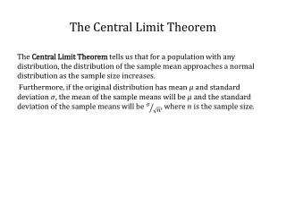
THE CENTRAL LIMIT THEOREM The “World is Normal” Theorem
But first,…Sampling Distribution of x When the Population Can Be Modeled with a Normal Model n=10 Sampling distribution of x: N( , /10) /10 Population distribution: N( , )
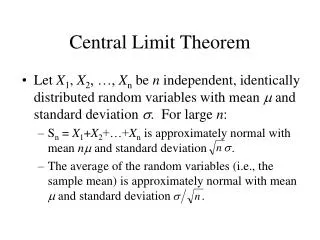
Normal Populations For example: • Important Fact: • The shape of the sampling distribution of the sample mean xis normal when the population from which the sample is selected is normal. This is true for any sample size n.
But Not All Populations Can Be Modeled by a Normal Model • What can we say about the shape of the sampling distribution of x when the population from which the sample is selected is not normal? http://bit.ly/2hBGl8k
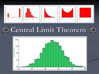
The Central Limit Theorem(for the sample mean x) • If a random sample of n observations is selected from a population (any population), then when n is sufficiently large, the sampling distribution of x will be approximately normal. (The larger the sample size, the better will be the normal approximation to the sampling distribution of x.)
The Importance of the Central Limit Theorem • When we select simple random samples of size n, the sample means will vary from sample to sample. We can model the distribution of these sample means with a probability model that is …
How Large Should n Be? • For the purpose of applying the Central Limit Theorem, we will consider a sample size to be large when n > 30. Even if the population from which the sample is selected looks like this … ← ← ← … the Central Limit Theorem tells us that a good model for the sampling distribution of the sample mean x is … → → →
Summary Population: mean ; stand dev. ; shape of population dist. is unknown; value of is unknown; select random sample of size n; Sampling distribution of x: mean ; stand. dev. /n; always true! By the Central Limit Theorem: the shape of the sampling distribution is approx normal, that is x ~ N(, /n)
The Central Limit Theorem(for the sample proportion p ) • If x “successes” occur in a random sample of n observations selected from a population (any population), then when n is sufficiently large, the sampling distribution of p =x/n will be approximately normal. (The larger the sample size, the better will be the normal approximation to the sampling distribution of p.)
The Importance of the Central Limit Theorem • When we select simple random samples of size n from a population with “success” probability p and observe x “successes”, the sample proportions p =x/n will vary from sample to sample. We can model the distribution of these sample proportions with a probability model that is…
How Large Should n Be? • For the purpose of applying the central limit theorem, we will consider a sample size n to be large when np ≥10 and n(1-p) ≥ 10 If the population from which the sample is selected looks like this … ← ← ← … the Central Limit Theorem tells us that a good model for the sampling distribution of the sample proportion is … → → →
Population Parameters and Sample Statistics • The value of a population parameter is a fixed number, it is NOT random; its value is not known. • The value of a sample statistic is calculated from sample data • The value of a sample statistic will vary from sample to sample (sampling distributions)
Example 2 • The probability distribution of 1-month incomes of experienced account executives has mean $20,000 and standard deviation $5,000. • a) A single executive’s 1-month income is $20,000. Can it be said that this executive’s income exceeds 50% of all account executive incomes? ANSWER No. P(X<$20,000)=? No information given about shape of distribution of X; we do not know the median of 1-month incomes.
Example 2(cont.) • b) n=64 experienced account executives are randomly selected. What is the probability that the sample mean exceeds $20,500?
Example 3 A sample of size n=16 is selected from a normally distributed population with E(X)=20 and SD(X)=8.
Example 3 (cont.) • c. Do we need the Central Limit Theorem to solve part a or part b? • NO. We are given that the population is normal, so the sampling distribution of the mean will also be normal for any sample size n. The CLT is not needed.
Example 4 • Battery life X~N(20, 10). Guarantee: avg. battery life in a case of 24 exceeds 16 hrs. Find the probability that a randomly selected case meets the guarantee.
Example 5 Cans of salmon are supposed to have a net weight of 6 oz. The canner says that the net weight is a random variable with mean =6.05 oz. and stand. dev. =.18 oz. Suppose you take a random sample of 36 cans and calculate the sample mean weight to be 5.97 oz. • Find the probability that the mean weight of the sample is less than or equal to 5.97 oz.
Population X: amount of salmon in a canE(x)=6.05 oz, SD(x) = .18 oz • X sampling dist: E(x)=6.05 SD(x)=.18/6=.03 • By the CLT, X sampling dist is approx. normal • P(X 5.97) = P(z [5.97-6.05]/.03) =P(z -.08/.03)=P(z -2.67)= .0038 • How could you use this answer?
Suppose you work for a “consumer watchdog” group • If you sampled the weights of 36 cans and obtained a sample mean x 5.97 oz., what would you think? • Since P( x 5.97) = .0038, either • you observed a “rare” event (recall: 5.97 oz is 2.67 stand. dev. below the mean) and the mean fill E(x) is in fact 6.05 oz. (the value claimed by the canner) • the true mean fill is less than 6.05 oz., (the canner is lying ).
Example 6 • X: weekly income. E(X)=1050, SD(X) = 100 • n=64; Xsampling dist: E(X)=1050 SD(X)=100/8 =12.5 • P(X 1022)=P(z [1022-1050]/12.5) =P(z -28/12.5)=P(z -2.24) = .0125 Suspicious of claim that average is $1050; evidence is that average income is less.
Example 7 • 12% of students at NCSU are left-handed. What is the probability that in a sample of 100 students, the sample proportion that are left-handed is less than 11%?
Too Heavy for the Elevator? • Mean weight of US men is 190 lb, thestandard deviation is 59 lb. A large freight elevator has a weight limit of 6600 lb. Find the probability that 30 men in the elevator will exceed the weight limit. • 30 men over 6600 lb.; • so the mean weight of the 30 men must be greater than 6600/30 = 220 lb.
Too Heavy for the Elevator? • X=weight of individual male; • E(X) = 190, SD(X) = 59 • Shape of probability distribution of X? Don’t know. • Sampling distribution of sample mean (n =30) • By the Central Limit Theorem, the sampling distribution of is approximately Normal!
Too Heavy for the Elevator? • Conclusion: There is only a 0.0026 chance that the 30 men will exceed the elevator’s weight limit.