Download

1 / 37
370 likes | 553 Views
Central Limit Theorem. So far, we have been working on discrete and continuous random variables. But most of the time, we deal with ONE random variable at a time. For example, if a random variable X follows a normal distribution, then ……. How about we have more than one random variable?

E N D
So far, we have been working on discrete and continuous random variables. • But most of the time, we deal with ONE random variable at a time. • For example, if a random variable X follows a normal distribution, then ……
How about we have more than one random variable? • For example, if a random variable Y is the sum of several random variables, X1 X2, …, Xn? And we want to work on Y. • That is to say, we want to find the pdf/cdf for Y, calculate probabilities under Y and find E(Y) and Var(Y).
Can we do that? • Yes: Most of the questions like that can be handled using probability theory. • Some simple examples: • If X1, X2, …, Xn are all Bernoulli r.v. with the same parameter p, then Y will be a binomial r.v. with parameters (n, p). • If X1, X2, …, Xn are all normal r.v. with the same mean μ and variance σ2 , then Y will be a normal r.v. with mean nμ and variance nσ2.
However • However, the sum of many other r.v. are beyond the range of this course. • Example: • If X1, X2, …, Xn are all exponential r.v. with parameter lambda, what is the distribution of Y? (this question actually has an answer, but we do not cover it in this course).
However • We should be able to work on most cases under some conditions: • The most important condition is: independence. • Example, given several independnet random variables, X1, X2, …, Xn, what can we do about their sum, S, or their mean, , where
To make it more general • Given independent random variables, X1, X2, …, Xn, what can we say about any linear combination in the form of a1X1+a2X2+…+anXn, where not all ai’s are zero. • We can see that both the sum, S, and the mean, are linear combinations of X1, X2, …, Xn.
Think about normal approximation to binomial example • A hotel has 100 rooms and the probability that a room is occupied at any given night is 0.6. We are interested in the number of rooms occupied each night. For example, what is the probability that there are more than 50 rooms occupied each night?
We can consider each room follows a Bernoulli distribution with parameter p=0.6. • The 100 rooms then have the same distribution with the same mean (p=0.6) and variance (p*(1-p)=0.24). • The total number of rooms occupied each night is just the sum of the 100 Bernoulli random variables, which is a binomial r.v. with parameters (100, 0.6)
We can calculate the probability of interest using binomial distribution. Let Xi be the outcome that each room is occupied or not and X be the total number of rooms occupied per night, then X=X1+X2+…+X100, and X~BIN(100, 0.6) • P(X>50)=1-P(X ≤50)=1-[P(X=0)+P(X=1)+…+P(X=50)] or =P(X=51)+P(X=52)+…+P(X=100) • That is a workable problem but requires a lot of calculation.
Normal approximation to Binomial • Alternatively, we can approximate the total number of rooms occupied each night by a normally distributed r.v., that is what we have talked about, normal approximation to binomial r.v.. • First, n*p=100*0.6=60>5 and n*(1-p)=100*0.4=40>5. • Since E(X)=100*0.6 and Var(X)=100*0.24, we can say X is approximately normally distributed with mean 60 and variance 24. • ThereforeP(X>50.5)=1-P(X<49.5)=1- Φ [(49.5-60)/sqrt(24)]=1- Φ(-0.4375)=1-0.33=0.67 • *** Don’t forget the continuity correction!!!
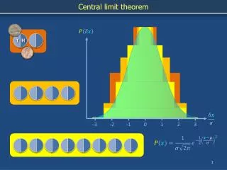
Now we know that the sum of several Bernoulli random variables, binomial, can be approximated by a normal random variable under some conditions, how about the other random variables? • We do have an answer to that… There is Binomial distribution for the sum of independent Bernoulli random variables, for anything else, we have central limit theorem.
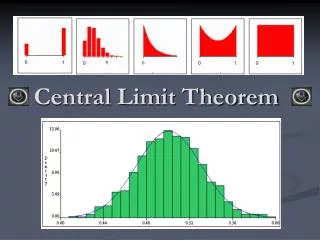
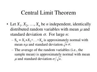
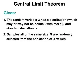
Central Limit Theorem • Suppose X1, X2, …, Xn are any independent random variables, each with mean μ1 ,μ2 , …, μn and variances σ12 ,σ22,…, σn2 ,then for arbitrary non-zero constants a1, a2, …, an, if n is large enough, • a1X1+a2X2+…+anXn is approximatelynormally distributed with mean a1μ1+a2µ2+…+anµn • and variance a21σ21+a22σ22+…+a2nσ2n.
More specifically • If X1, X2, …, Xn are any independent random variables with the same mean, μ and variance σ2 , the sum and mean of all X’s are approximately normally distributed • Sn~N(nµ, nσ2) and ~ N(µ, σ2/n), if n is large enough.
How large is large enough? Usually, we think n is large enough if n is 30 or more.
Example I • Suppose state i has 82 counties and let Xi be the number of car accidents each month in county i. We can assume that all Xi’s are independent and they all follow a Poisson distribution with mean 3.
Example I contd. • A. Some researchers are interested in, Xt, the total number of car accidents in the five neighboring counties of the state capital. What is the probability distribution for Xt and what is the probability that there are more than 20 car accidents in those five counties last month?
Example I Contd. • We know that the sum of n independent Poisson random variables with parameter λ follows a Poisson distribution with parameter nλ. Therefore, we have Xt~Poi(15). • P(Xt>20)=1-P(Xt ≤ 20) • =1-[P(Xt=0)+P(Xt=1)+…P(Xt=20)] • =1-0.917 • =0.083
Example I • B. Some other researchers are interested in the total number of car accidents each month in this state. They want to find an approximation of the probability that there are less than 250 car accidents in the state last month. How can they do that?
Example I Contd. • This time, since we are interested in the sum of car accidents per month for 82 counties, which is greater than 30, we can use the CLT to get an approximate result. • Since all Xi~Poi(3), Sn=X1+X2+…+X82 can be approximated by a normal r.v. with mean 246 (3*82) and variance 246.(remember that the mean and variance of a Poisson r.v. are equal!!!)
Therefore, P(Sn<249.5)= Φ [Z<(249.5-246)/sqrt(246)] • = Φ [0.22]=0.5871 • Again, there is continuity correction since Poisson is discrete and Normal is continuous.
Example II • An automobile company manufactured two batches of car engines of 100 each. The life of the engines in batch 1 is evenly distributed between 8 and 20 years while the life of batch 2 engines follows an exponential distribution with mean 14 years. Think about the average life of these two batches. On average, which batch has a higher probability of lasting more than 15 years ?
Example II • To be clear, the random variable of interest in this problem is the mean life of the engines in the two batches.
For batch 1, since the life of each engine follows a uniform distribution (we see that from the word “evenly ”), it has a mean of (8+20)/2=14 years and variance (20-8)2/12=12. • Also, since we have 100 independent engines, we can use the CLT. • Therefore, the mean life of engines in batch 1 can be approximated by a normal r.v. with mean 14 and variance 12/100=0.12
P(X>15)=1-P(X<15) • =1- P(Z<(15-14)/sqrt(0.12)) • =1- Φ (2.8867) • = 1- 0.9981 • =0.0019
For batch 2, since the life of each engine follows an exponential distribution with mean of 14, then we know its mean is 14 and variance is 196 (142). • Therefore, the mean life of engines in batch 2 can be approximated by a normal distribution with mean 14 and variance 196/100=1.96.
P(X>15)=1-P(X<15) • =1- P(Z<(15-14)/sqrt(1.96)) • =1- Φ (0.7143) • =1-0.7611 • =0.2389
Implication of CLT for Statistics • In statistics, we usually consider, for each subject in the population, the numeric representation of the characteristics of interest follow the same distribution. • If we have a simple random sample, (SRS), of size n, we consider those n subjects in our sample also follow the same distribution since they are from the same population. • Therefore, the mean of the sample, (if the sample size is large enough, say >30), is considered approximately normally distributed. Also, we can find a relationship between the mean and variance of the sample and the population.
Implication of CLT for Statistics • Assuming we have collected a simple random sample. There are a couple of things that we need to put together. • 1. The purpose of collecting and studying the sample is to study the population, for example, population mean. • 2. We assume all the subjects in the SRS follow the same distribution. • 3. Therefore, regardless of the distribution of each individual subject, we know that the mean of the sample is approximately normally distributed. • 4. Then we will use what we know about the sample mean to answer questions about the population mean. But apparently, the sample mean itself is not enough, what to do next? We will talk about it later.
Light Bulb Example • Tim has a lamp at his desk. He just spotted a clearance sale on the bulbs for his lamp and purchased 100 of them. He plans to replace the bulb immediately after one dies and hopes that his bulbs can last for more than 10 years. Each of the bulbs’ life follows an exponential distribution with a mean life of 800 hours. If we assume 365 days for each year, what is the probability that Tim’s 100 bulbs can last more than 10 years.
Light Bulb Example • In this example, we are interested in the total life of Tim’s 100 bulbs (since he will replace one immediately after it dies). • Let Xi be the life of each bulb and we are interested in S=X1+X2+…+X100. We want to find the probability, P(S>10 years). • Some translations are needed. The life of each bulb is measured in hours, so we must translate 10 years into hours, (assuming 365 days a year), which gives us 10*365*24=87600. • Therefore, the probability of interest is P(S>87600)
Light Bulb Example • Now let’s think about the distribution of S. • 1. S is the sum of all Xi’s • 2. Each Xi ~ EXP(800), or E(Xi)=800, Var(Xi)=800^2 • 3. There are 100 Xi’s • Therefore, according to CLT, S can be approximated by a normal r.v. with mean 100*800 and variance 100*(800^2)
Light Bulb Example Finally, we need to calculate P(S > 87600 ) = 1 – P(P < 87600) = 1 – P [ Z < (87600-80000)/sqrt(100*800^2) ] = 1 – P [ Z < 7600/8000 ] = 1 – P [ Z < 0.95 ] =1-0.8289 =0.1711 Finally, we say that there is about 17% chance that Tim’s 100 bulbs will last more than 10 years.
Brake Warranty Example • A manufacturer makes a type of brakes whose life follows an exponential distribution with a mean life of 3 years. A car dealership has 20 cars on their parking lot with that kind of brake. The dealership is considering selling a one-year warranty on the brakes for their car. They decide that they will only do it if less than 20 brakes will need work within the warranty period. What is the probability that the dealership will offer that warranty?
Brake Warranty Example • In this example, the variable, call it T, that will affect the dealership’s decision is the number of brakes that will need work within 1 year. • 2. For each brake, it may need work within 1 year with some probability p, that makes it a Bernoulli r.v. with parameter p. We assume that p is the same for all the brakes on the dealer’s cars, therefore, T will be a binomial r.v. with parameters n and p. • 3. There are 4 brakes on each car so we are actually talking about 20*4=80 brakes. We then have n=80. But what is p?
Brake Warranty Example • Each brake’s life follows an exponential distribution with mean 3. Let Xi be the time until this brake needs work, then p=P(Xi<1)=1-exp(-1/3) =0.2835 • Therefore, T~BIN(80, 0.2835). • 80*p=22.67750 > 5 and 80*(1-p)=57.32 > 5 • Then T can be approximated by a normal r.v. with mean 22.68 and variance 16.25.
The dealership will offer the warranty if T<20, the probability is • P(T<20) • =P((T-22.68)/sqrt(16.25) < (19.5-22.68)/sqrt(16.25)) • =P(Z< -0.79 ) • =0.2148 • That tells us that there is only about 21% chance that the dealer will offer the warranty on the brakes.