Download
1 / 9
90 likes | 107 Views
1/16/2014. 7.3B The Central Limit Theorem. Section 7.3 Sampling Distributions & The CLT. Learning Objectives. After this section, you should be able to… APPLY the central limit theorem to help find probabilities involving a sample mean. Sample Means. The Central Limit Theorem

E N D
1/16/2014 7.3B The Central Limit Theorem
Section 7.3Sampling Distributions & The CLT Learning Objectives After this section, you should be able to… • APPLY the central limit theorem to help find probabilities involving a sample mean
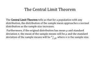
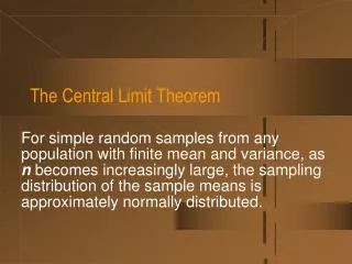
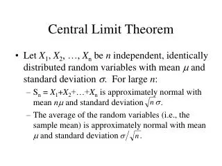
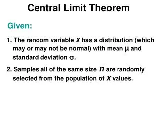
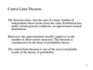
Sample Means • The Central Limit Theorem Most population distributions are not Normal. What is the shape of the sampling distribution of sample means when the population distribution isn’t Normal? It is a remarkable fact that as the sample size increases, the distribution of sample means changes its shape: it looks less like that of the population and more like a Normal distribution! When the sample is large enough, the distribution of sample means is very close to Normal, no matter what shape the population distribution has, as long as the population has a finite standard deviation. Definition: Note: How large a sample size n is needed for the sampling distribution to be close to Normal depends on the shape of the population distribution. More observations are required if the population distribution is far from Normal.
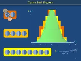
Sample Means • The Central Limit Theorem Consider the strange population distribution from the Rice University sampling distribution applet. Describe the shape of the sampling distributions as n increases. What do you notice? Normal Condition for Sample Means
Example: Mean Texts Suppose that the number of texts sent during a typical day by a randomly selected high school student follows a right-skewed distribution with a mean of 15 and a standard deviation of 35. Assuming that students are your high school are typical texters, how likely is it that a random sample of 50 students will have sent more than a total of 1000 texts in the last 24 hours? Use the 4 Step Process! Sample Means State: I want to find the probability that the total number of texts in the last 24 hours is greater than 1000 for a random sample of 50 high school students. Plan: A total of 1000 texts among 50 students is the same as an average number of 20 texts. Since n is large (50>30), the distribution of x-bar is approximately Normal. Do: We need to find P(mean number of texts> 20 texts). Conclude: There is about a 16% chance that a random sample of 50 high school students will send more than 1000 texts in a day.
Example: Servicing Air Conditioners Based on service records from the past year, the time (in hours) that a technician requires to complete preventative maintenance on an air conditioner follows the distribution that is strongly right-skewed, and whose most likely outcomes are close to 0. The mean time is µ = 1 hour and the standard deviation is σ = 1 Sample Means Your company will service an SRS of 70 air conditioners. You have budgeted 1.1 hours per unit. Will this be enough? Use the 4 Step Process! Since the 10% condition is met (there are more than 10(70)=700 air conditioners in the population), the sampling distribution of the mean time spent working on the 70 units has The sampling distribution of the mean time spent working is approximately N(1, 0.12) since n = 70 ≥ 30. We need to find P(mean time > 1.1 hours) If you budget 1.1 hours per unit, there is a 20% chance the technicians will not complete the work within the budgeted time.
Section 7.3Sample Means Summary In this section, we learned that…
Section 7.3Sample Means Summary In this section, we learned that…
Homework: • Chapter 7: p.454 #57-63 odd, 65-68