Download
1 / 38
380 likes | 530 Views
The paired sample experiment. The paired t test. Frequently one is interested in comparing the effects of two treatments (drugs, etc…) on a response variable. The two treatments determine two different populations Popn 1 cases treated with treatment 1.

E N D
The paired sample experiment The paired t test
Frequently one is interested in comparing the effects of two treatments (drugs, etc…) on a response variable. The two treatments determine two different populations • Popn 1 cases treated with treatment 1. • Popn 2 cases treated with treatment 2 The response variable is assumed to have a normal distribution within each population differing possibly in the mean (and also possibly in the variance)
Two independent sample design A sample of size ncases are selected from population 1 (cases receiving treatment 1) and a second sample of size mcases are selected from population 2 (cases receiving treatment 2). The data • x1, x2, x3, …, xn from population 1. • y1, y2, y3, …, ym from population 2. The test that is used is the t-test for two independent samples
The matched pair experimental design (The paired sample experiment) Prior to assigning the treatments the subjects are grouped into pairs of similar subjects. Suppose that there are nsuch pairs (Total of 2n = n + n subjects or cases), The two treatments are then randomly assigned to each pair. One member of a pair will receive treatment 1, while the other receives treatment 2. The data collected is as follows: • (x1, y1), (x2 ,y2), (x3 ,y3),, …, (xn, yn) . xi = the response for the case in pair i that receives treatment 1. yi = the response for the case in pair i that receives treatment 2.
Let di = yi - xi. Then d1, d2, d3 , … , dn Is a sample from a normal distribution with mean, md =m2 – m1 , and variance standard deviation Note if the x and y measurements are positively correlated (this will be true if the cases in the pair are matched effectively) thansd will be small.
To test H0: m1 = m2 is equivalent to testing H0: md = 0. (we have converted the two sample problem into a single sample problem). The test statistic is the single sample t-test on the differences d1, d2, d3 , … , dn namely df = n - 1
Example We are interested in comparing the effectiveness of two method for reducing high cholesterol The methods • Use of a drug. • Control of diet. The 2n = 8 subjects were paired into 4 match pairs. In each matched pair one subject was given the drug treatment, the other subject was given the diet control treatment. Assignment of treatments was random.
Differences for df = n – 1 = 3, Hence we accept H0.
Many statistical procedures make assumptions The t test, z test make the assumption that the populations being sampled are normally distributed. (True for both the one sample and the two sample test).
This assumption for large sample sizes is not critical. (Reason: The Central Limit Theorem) The sample mean, the statistic z will have approximately a normal distribution for large sample sizes even if the population is not normal.
For small sample sizes the departure from the assumption of normality could affect the performance of a statistical procedure that assumes normality. For testing, the probability of a type I error may not be the desired value of a= 0.05 or 0.01 For confidence intervals the probability of capturing the parameter may be the desired value (95% or 99%) but a value considerably smaller
Example: Consider the z-test For a= 0.05 we reject the hypothesized value of the mean if z < -1.96 or z > 1.96 Suppose the population is an exponential population with parameter l. (m= 1/land s = 1/l)
Actual population Assumed population
Suppose the population is an exponential population with parameter l. (m= 1/land s = 1/l) It can be shown that the sampling distribution of is the Gamma distribution with Use mgf’s The distribution of is not the normal distribution with
Sampling distribution of Actual distribution n = 2 Distribution assuming normality
Sampling distribution of Actual distribution n = 5 Distribution assuming normality
Sampling distribution of Actual distribution n = 20 Distribution assuming normality
Definition When the data is generated from process (model) that is known except for finite number of unknown parameters the model is called a parametric model. Otherwise, the model is called a non-parametric model Statistical techniques that assume a non-parametric model are called non-parametric.
The sign test A nonparametric test for the central location of a distribution
We want to test: H0: median = m0 against HA: median m0 (or against a one-sided alternative)
The assumption will be only that the distribution of the observations is continuous. • Note for symmetric distributions the mean and median are equal if the mean exists. • For non-symmetric distribution, the median is probably a more appropriate measure of central location.
The Sign test: • The test statistic: S = the number of observations that exceed m0 Comment: If H0: median =m0 is true we would expect 50% of the observations to be above m0, and 50% of the observations to be below m0,
If H 0 is true then S will have a binomial distribution with p = 0.50, n = sample size. 50% 50% median = m0
If H 0 is not true then S will still have a binomial distribution. However p will not be equal to 0.50. m0 > median p< 0.50 p median m0
m0 < median p> 0.50 p median m0 p= the probability that an observation is greater than m0.
Summarizing: If H0 is true then S will have a binomial distribution with p = 0.50, n = sample size. n = 10
The critical and acceptance region: n = 10 Choose the critical region so that a is close to 0.05 or 0.01. e. g. If critical region is {0,1,9,10} then a= .0010 + .0098 + .0098 +.0010 = .0216
e. g. If critical region is {0,1,2,8,9,10} then a= .0010 + .0098 +.0439+.0439+ .0098 +.0010 = .1094 n = 10
If one can’t determine a fixed confidence region to achieve a fixed significance level a, one then randomizes the choice of the critical region • In the example with n = 10, if the critical region is {0,1,9,10} then a= .0010 + .0098 + .0098 +.0010 = .0216 • If the values 2 and 8 are added to the critical region the value of increases to 0.216 + 2(.0439) = 0.0216 + 0.0878 = 0.1094 • Note 0.05 =0.0216 + 0.3235(.0878) Consider the following critical region • Reject H0 if the test statistic is {0,1,9,10} • If the test statistic is {2,8} perform a success-failure experiment with p = P[success] = 0.3235, If the experiment is a success Reject Ho. • Otherwise we accept H0.
Example Suppose that we are interested in determining if a new drug is effective in reducing cholesterol. Hence we administer the drug to n = 10 patients with high cholesterol and measure the reduction.
The data Let S = the number of negative reductions = 2
If H0 is true then S will have a binomial distribution with p = 0.50, n = 10. We would expect S to be small if H0 is false. n = 10
Choosing the critical region to be {0, 1, 2} the probability of a type I error would be a = 0.0010 + 0.0098 + 0.0439 = 0.0547 Since S = 2 lies in this region, the Null hypothesis should be rejected. Conclusion: There is a significant positive reduction (a= 0.0547) in cholesterol.
If n is large we can use the Normal approximation to the Binomial. Namely S has a Binomial distribution with p = ½ and n = sample size. Hence for large n, S has approximately a Normal distribution with mean and standard deviation
Hence for large n,use as the test statistic (in place of S) Choose the critical region for z from the Standard Normal distribution. i.e. Reject H0 if z < -za/2 or z > za/2 two tailed ( a one tailed test can also be set up.