Download

1 / 31
330 likes | 460 Views
Hypothesis tests I . One - sample t -test , paired t-test. Motivating example. Two lecturers argue about the mean age of the first year medical students. Lecturer#1 claims that the mean age of the first year medical students is 20. Lecturer#2 does not agree. Who is right?

E N D
Motivating example • Two lecturers argue about the mean age of the first year medical students. • Lecturer#1 claims that the mean age of the first year medical students is 20. • Lecturer#2 does not agree. • Who is right? • Statistically speaking: the population is the set of ALL first year medical students (anywhere, any time). • Lecturer#1 claims that the population mean μ=20. • Lecturer#2 claims that the population mean μ ≠ 20
How to find the answer • To be sure, we have two know the age of the TOTAL population (impossible) • To be confident, we draw a sample from the population (i.e., get the age of some first year medical students). n=137 • Calculate mean age of the sample • If the sample is representative, we believe that the sample mean approximates the population mean • To be 95% confident, calculate the 95% confidence interval for the population mean (20.35-21.39) • With 95% probability, the true population mean (i.e. the mean age of the first year medical students) lies somewhere between 20.35 and 21.39.
Review: interval estimate, confidence interval (CI) • Confidence interval: an interval which contains the value of the (unknown) population parameter with high probability. • The probability assigned is the confidence level (generally: 0.90, 0.95, 0.99 ) • Most often used confidence level: 0.95 (95%) • Level of „mistake” or „error”: =1-0.95=0.05 (5%)
Formula of the confidence interval for the normal population’s mean μwhen is unknown • n=t/2 is the two-tailed critical value of the Student's t statistic with n-1 degrees of freedom
Calculation of the confidence interval for the population’s mean μfor the example • Let the sample be the data of the questionnaire filled in by students at the first lecture. • We calculated the sample characteristics • n=137 • Sample mean=20.87 • Sample SD=3.071
Calculation of the confidence interval for the population’s mean μfor the example • n=137 • df=136 (degrees of freedom • sample mean • SD=3.071 • t/2= 1.977 (from the table) • Lower limit: 20.87-0.518=20.352 • Upper limit: 20.87+0.518=21.388 • 95%CI: (20.35-21.39)
Hypothesis testing • Hypothesis: a statement about the population • Based on our data (sample) we conclude to the whole phenomenon (population) • We examine whether our result (difference in samples) is greater then the difference caused only by chance.
Hypothesis • Hypothesis: a statement about the population • Examples • H1: p=0.5 (a coin is fair - half the flips would result in Heads and half, in Tails) • H2: p≠0.5 ( a coin is not fair) • H3: =20 (the population mean is 19) • H4: ≠20 (the population mean is not 12) • Statisticians usually test the hypothesis which tells them what to expect by giving a specific value to work with. They refer to this hypothesis as the null hypothesis and symbolize it as H0. The null hypothesis is often the one that assumes fairness, honesty or equality. • The opposite hypothesis is called alternative hypothesis and is symbolized by Ha. This hypothesis, however, is often the one that is of interest.
Steps of hypothesis-testing • Step 1. State the motivated (alternative) hypothesis Ha. • Step 2. State the null hypothesis H0. • Step 3. Select the , the probability of Type I error, or the α significance level. α =0.05 or α =0.01. • Step 4. Choose the size n of the random sample • Step 5.Select a random sample from the appropriate population and obtain your data. • Step 6. Calculate the decision rule –it depends on problem, assumptions, type of data, etc... • Step 7. Decision. • a) Reject the null hypothesis and claim that the alternative hypothesis was correct the difference is significant at α100% level. • b) Fail to reject the null hypothesis correct the difference is not significant at α 100% level .
Testing the mean of a sample drawn from a normal population for the data of the example • Step 1-2. State null and the alternative hypotheses • H0: =20 , Ha: 20 • Step 3. Select the , the probability of Type I error, or the α significance level. • α =0.05 • Step 4-5. Choose the size n of the random sample and select a random sample from the appropriate population and obtain your data. • Step 6. Calculate the decision rule – now: confidence interval • Calculate the 95% confidence interval for the population mean: (20.35-21.39). • With 95% probability, the true population mean (i.e. the mean age of the first year medical students) lies somewhere between 20.35 and 21.39. • Decision rule: check whether the hypothesised mean (20) is in the interval or not • Step 7. Decision. • 20 is not in the interval so we reject the null hypothesis and claim that the alternative hypothesis was correct the difference is significant at 5% level. .
Testing the mean of a sample drawn from a normal population: one-sample t-test (general)Decision rule based on confidence interval • Step 1-2. State null and the alternative hypotheses • H0: =c , Ha: c, c is a given constant • Step 3. You select the , the probability of Type I error, or the α significance level. • α =0.05 • Step 4-5. You choose the size n of the random sample and select a random sample from the appropriate population and obtain your data. • Step 6. Calculate the decision rule. • Calculate the 95% confidence interval for the population mean. Decision rule: check whether the hypothesised mean (c) is in the interval or not • Step 7. Decision. • a) if c is not in the interval, we reject the null hypothesis and claim that the alternative hypothesis was correct the difference is significant at 5% level. • b) if c is in the interval, we fail to reject the null hypothesis (we accept it) and claim that your null hypothesis was correct, the difference is not significant at 5% level.
Step 1-2. H0: =20 , Ha: 20 Step 3. α =0.05 Step 4-5. You choose the size n of the random sample and select a random sample from the appropriate population and obtain your data. Step 6. Calculate the decision rule. Calculate the test-statistic: If H0 is true, this test-statistic has a t-distribution with n-1 degrees of freedom. The acceptance (non-rejection) region is the set of values for which we accept the null hypothesis (- 1.977, 1.977) The critical region (rejection region) is the set of values for which the null hypothesis is rejected. Decision rule: check whether the calculated t-value (t) is in the acceptance interval or not Step 7. Decision: as t=3.321 is not in the acceptance region,3.321>1.977, |t|>ttable, the difference is significant at 5% level Testing the mean of a sample drawn from a normal population: one-sample t-test Decision rule based on t-value Acceptance interval t=3.321
Step 1-2. H0: =c , Ha: c c is a given constant Step 3. α =0.05 Step 4-5. You choose the size n of the random sample and select a random sample from the appropriate population and obtain your data. Step 6. Calculate the decision rule. Calculate the test-statistic: If H0 is true, this test-statistic has a t-distribution with n-1 degrees of freedom. The acceptance (non-rejection) region is the set of values for which we accept the null hypothesis (- ttable, ttable) The critical region (rejection region) is the set of values for which the null hypothesis is rejected. Decision rule: check whether the calculated t-value (t) is in the acceptance interval or not Step 7. Decision: if t is not in the acceptance region (t> ttable or t< - ttable, i.e, |t|>ttable ),, the difference is significant at α level if t is in the acceptance region (- ttable<t< ttable, i.e. |t|<ttable), the difference is not significant at α level Testing the mean of a sample drawn from a normal population: one-sample t-test (general)Decision rule based on t-value Acceptance region tcalc
Step 1-2. H0: =19 , Ha: 19 Step 3. α =0.05 Step 4-5. Choose the size n of the random sample and select a random sample from the appropriate population and obtain your data. Step 6. Calculate the decision rule. Calculate the test-statistic: If H0 is true, this test-statistic has a t-distribution with n-1 degrees of freedom. The acceptance (non-rejection) region is the set of values for which we accept the null hypothesis (- 1.977, 1.977) p-value=the two tailed tail area under the curve cut by our calculated t-value Step 7. Decision: as p=0.001152<0.05, the difference is significant at 5% level Testing the mean of a sample drawn from a normal population: one-sample t-test Decision rule based on p-value Acceptance interval t=3.321 p=.001152
Step 1-2. H0: =19 , Ha: 19 Step 3. α =0.05 Step 4-5. Choose the size n of the random sample and select a random sample from the appropriate population and obtain your data. Step 6. Calculate the decision rule. Calculate the test-statistic (tcalc) If H0 is true, this test-statistic has a t-distribution with n-1 degrees of freedom. p-value=the two tailed tail area under the curve cut by our calculated t-value Step 7. Decision: If p<, we decide that the difference is significant at 100% level If p>, we decide that the difference is not significant at 100% level Testing the mean of a sample drawn from a normal population: one-sample t-test Decision rule based on p-value (general) Acceptance interval ttable tcalc p=.001152
Summary of the equivalent decision rules for one-sample t-testAssumption: normality (the sample is drawn from a normal distribution)
SPSS result To decide based on t-value and degrees of freedom, we need a t-table p-value, If p<, the difference is significant, If p<, the difference is not significant
One-sample t-test, example 2. • A company produces a 16 ml bottle of some drug (solution). The bottles are filled by an automated bottle-filling process. If this process is substantially overfilling or under filling bottles, then this process must be shut down and readjusted. Overfilling results in lost profits for the company, while under filling is unfair to consumers. For a given adjustment of the bottles consider the infinite population of all the bottle fills that could potentially be produced. We let denote the mean of the infinite population of all the bottle fills. • The company has decided that it will shut down and readjust the process if it can be very certain that the mean fill is above or below the desired 16 ml. • Now suppose that the company observes the following sample of n=6 bottle fills: • 15.68, 16.00, 15.61, 15.93, 15.86, 15.72 • It can be verified that this sample has mean=15.8 and standard deviation SD=0.156. • Question: Is it true that the mean bottle fill in the population is 16?
A one-sample t test for paired differences (paired t-test) • Self-control experiment • Related data: • Before treatment – after treatment • Left side – right side • Matched pairs • Null hypothesis: there is no treatment-effect, the difference is only by chance • HO: before= after or difference= 0 • Alternative hypothesis: there is a treatment effect • HA: before≠ after or difference≠ 0
A study was conducted to determine weight loss, body composition, etc. in obese women before and after 12 weeks of treatment with a very-low-calorie diet . We wish to know if these data provide sufficient evidence to allow us to conclude that the treatment is effective in causing weight reduction in obese women. The mean difference is actually 4. Is it a real difference? Big or small? If the study were to be repeated, would we get the same result or less, even 0? Before After Difference 85 86 -1 95 90 5 75 72 3 110 100 10 81 75 6 92 88 4 83 83 0 94 93 1 88 82 6 105 99 6 Mean 90.8 86.8 4. SD 10.79 9.25 3.333 Paired t-test, example
Paired t-test, example (cont). • Idea: if the treatment is not effective, the mean sample difference is small (close to O), if it is effective, the mean difference is big. • HO: before= after or difference= 0 (c=0)!! • HA: before≠ after or difference≠ 0 • Let =0. • Degrees of freedom=10-1=9, • ttable=t0.05,9=2.262 • Mean=4, SD=3.333 • SE=3.333/10=1.054
Paired t-test, example (cont.) • Decision based on confidence interval: • 95%CI:(4-2.262*1.054, 4+2.262*1.054)=(1.615, 6.384) • If H0 were true, 0 were inside the confidence interval • Now 0 is outside the confidence interval, the difference is significant at 5% level, the treatment was effective. • The mean loss of body weight was 4 kg, which could be even 6.36 but minimum 1.615, with 95% probability.
Decision based on test statistic (t-value): • This t has to be compared to the critical t-value in the table. • |t|=3.795>2.262(=t0.05,9), the difference is significant at 5% level • Decision based on p-value: • p=0.004, p<0.05, the difference is significant at 5% level Acceptance region tcomputed, test statistic ttable, critical value
Example from the medical literatureV. Lindén: Vitamin D and Myocardial Infarction. BMJ 1974,3,647-650
Review questions and problems • What is a hypothesis • Null-and alternative hypothesis • Steps of hypothesis testing • The null- and alternative hypothesis of the one-sample t-test • The assumption of the one-sample t-test • Decision rules of the one-sample t-test • Testing significance based on a confidence interval • Testing significance based on t-statistic • Testing significance based on p-value • Meaning of the p-value • In a study, systolic blood pressure of 10 healthy women was measured. The mean was 119, the standard error 0.664. Supposing that this sample was drawn from a normal distribution, check whether the population mean is 125! (=0.05, ttable=2.26). • To test the effect of a new drug, the systolic blood pressure was measured on the same 5 patients before and after the treatment. The mean of the differences is = 6, the standard error of the differences is SE=4.65. To test the effect of the drug, what is the appropriate test? Find the value of the test statistics and decide whether the difference is significant or not. ( =0.05, ttable=2.57)