Download
1 / 18
180 likes | 304 Views
Application of Generalized Extreme Value theory to coupled general circulation models. Michael F. Wehner Lawrence Berkeley National Laboratory mfwehner@lbl.gov SAMSI Climate Change Workshop February 17-19, 2010. Outline. GEV results in assessment reports Uncertainty in temperature extremes

E N D
Application of Generalized Extreme Value theory to coupled general circulation models Michael F. Wehner Lawrence Berkeley National Laboratory mfwehner@lbl.gov SAMSI Climate Change Workshop February 17-19, 2010
Outline • GEV results in assessment reports • Uncertainty in temperature extremes • Model fidelity and precipitation extremes • A few points for the discussion session
GEV results in assessment reports “Rare events will become commonplace”
Simulations for 2090-2099 indicating how currently rare extremes (a 1-in-20-year event) are projected to become more commonplace. a) Temperature - a day so hot that it is currently experienced once every 20 years would occur every other year or more by the end of the century. (Units:years)
Sources of uncertainty in estimating return values • 20 year return value of annual maximum daily mean surface air temperature • GEV parameters (Short sample size) • Unforced internal variability • Multi-model differences
GEV parameter uncertainty • Following the bootstrapping method of Hosking and Wallis • Fit GEV parameters to sample • Generate 50 random samples distributed by the GEV distribution • Calculate return values and their standard deviation • CCSM3.0 • 20 years • 40 years • 100 years • Average over • land (CMIP3 models)
Internal variability • Divide long control run into 40 year segments • Calculate return value for each segment and s CCSM3.0 600 years
Multi-model variation • Fifteen CMIP3 forty year control runs • Intermodel standard deviation Color scale is 5 times the previous two slides
Multi-model variation • Fifteen CMIP3 forty year control runs • Sam as previous except remove mean state bias Color scale is 5 times the previous two slides
Model resolution and extreme precipitation • Typical CMIP3 models are too coarse to simulate rare intense storms. • Horizontal resolution study with fvCAM2.2 • 200km (B mesh) • 100km (C mesh) • 50km (D mesh)
Model resolution and extreme precipitation • 20 year return value of annual maximum daily total precipitation (mm/day)
from the CCSP3.3 report • Simulations for 2090-2099 indicating how currently rare extremes (a 1-in-20-year event) are projected to become more commonplace. (b) daily total precipitation events that occur on average every 20 years in the present climate would, for example, occur once in every 4-6 years for N.E. North America. (Units:years)
Conclusions • IPCC AR5 will contain far more about extremes than AR4 • Largest source of uncertainty is inter-model difference • Uncertainty in the fit of GEV is about the same as unforced internal variability and is small! • Extreme precipitation requires high resolution. • At least over land. • Makes it hard to make projections with the CMIP3 models.
Discussion • GEV distribution fits climate data very well • Cells that fail the Anderson Darling test at 5% level • Surface air temperature annual maximum • Arctic failure is due to clustering at freezing point. Not very interesting, return value is 0oC.
Discussion • Detection & attribution of changes in extreme weather events • Zwiers et al GEV methodology: let location parameter be time dependent. Scale and shape parameters be static. Test whether time dependence is significant. • Temperature: Is this trivial if mean temperature changes have been detected and attributed? How does the difference between a return value and the mean change? • Precipitation: Widely believed to be more detectible due to Clausius-Clayperon relationship. But changes may not be of the same sign. May not be as severe as mean precipitation changes
Projected 1990-2090 DRV minus DTmean • SRES A1B (4 models) • Change is confined to land and fairly small (<2.5K) • Should we expect to detect this change in distribution shape?
1990-2090 wintertime precipitation changes SRES A1B 20 year return value mean x