Download

1 / 22
220 likes | 343 Views
Vector Generalized Additive Models and applications to extreme value analysis. Olivier Mestre (1,2) Météo-France, Ecole Nationale de la Météorologie, Toulouse, France Université Paul Sabatier, LSP, Toulouse, France Based on previous studies realized in collaboration with :

E N D
Vector Generalized Additive Modelsand applications to extreme value analysis Olivier Mestre (1,2) Météo-France, Ecole Nationale de la Météorologie, Toulouse, France Université Paul Sabatier, LSP, Toulouse, France Based on previous studies realized in collaboration with : Stéphane Hallegatte (CIRED, Météo-France) Sébastien Denvil (LMD)
SMOOTHER « Smoother=tool for summarizing the trend of a response measurement Y as a function of predictors » (Hastie & Tibshirani) estimate of the trend that is less variable than Y itself • Smoothing matrix S Y*=SY The equivalent degrees of freedom (df) of the smoother S is the trace of S. Allows compare with parametric models. • Pointwise standard error bands COV(Y*)=V=S tS ² given an estimation of ², this allows approximate confidence intervals (values : ±2square root of the diagonal of V)
SCATTERPLOT SMOOTHING EXAMPLE • Data: wind farm production vs numerical windspeed forecasts
SMOOTHING • Problems raised by smoothers How to average the response values in each neighborhood? How large to take the neighborhoods? Tradeoff between bias and variance of Y*
SMOOTHING: POLYNOMIAL (parametric) • Linear and cubic parametric least squares fits: MODEL DRIVEN APPROACHES
SMOOTHING: BIN SMOOTHER • In this example, optimum intervals are determined by means of a regression tree
SMOOTHING: RUNNING LINE • Running line
KERNEL SMOOTHER • Watson-Nadaraya
SMOOTHING: LOESS • The smooth at the target point is the fit of a locally-weighted linear fit (tricube weight)
CUBIC SMOOTHING SPLINES • This smoother is the solution of the following optimization problem: among all functions f(x) with two continuous derivatives, choose the one that minimizes the penalized sum of squares Closeness to the data penalization of the curvature of f It can be shown that the unique solution to this problem is a natural cubic spline with knots at the unique values xi Parameter can be set by means of cross-validation
CUBIC SMOOTHING SPLINES • Cubic smoothing splines with equivalent df=5 and 10
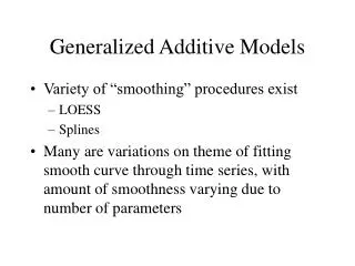
Additive models • Gaussian Linear Model : IE[Y]=o+1X1+2X2 • Gaussian Additive model : IE[Y]=S1(X1)+S2(X2) S1, S2 smooth functions of predictors X1, X2, usually LOESS, SPLINE Estimation of S1, S2 : « Backfitting Algorithm » • PRINCIPLE OF THE BACKFITTING ALGORITHM Y=S1(X1)+e estimation S1* Y-S1*(X1)=S2(X2)+e estimation S2* Y-S2*(X2)=S1(X1)+e estimation S1** Y-S1**(X1)=S2(X2)+e estimation S2** Y-S2**(X2)=S1(X1)+e estimation S1*** Etc… until convergence
Additive models • Additive models One efficient way to perform non-linear regression, but… • Crucial point ADAPTED WHEN ONLY FEW PREDICTORS 2, 3 predictors at most
Additive models • Philosophy DATA DRIVEN APPROACHES RATHER THAN MODEL DRIVEN APPROACH USEFUL AS EXPLORATORY TOOLS • Approximate inference tests are possible, but full inferences are better assessed by means of parametric models
Generalized Additive models (GAM) • Extension to non-normal dependant variables • Generalized additive models : additive modelling of the natural parameter of exponential family laws (Poisson, Binomial, Gamma, Gauss…). g[µ]==S1(X1)+S2(X2) • Vector Generalized Additive Models (VGAM): one step beyond…
Example 1 Annual umber and maximum integrated intensity (PDI) of hurricane tracks over the North Atlantic
Number of Hurricanes • Number of Hurricanes in North Atlantic ~ Poisson distribution
Factors influencing the number of hurricanes • GAM applied to number of hurricanes (YEAR,SST,SOI,NAO)
GAM model • Log()= o+S1(SST)+S2(SOI)
PARAMETRIC model • “broken stick model” (with continuity constraint) in SOI, revealed by GAM analysis • log() = o+SOI(1)SOI+SSTSST SOI<K = o+SOI(1)SOI+SOI(2)(SOI-K)+SSTSST SOIK • The best fit obtained for SOI value K=1 log-likelihood=-316.16, to be compared with -318.71 (linearity) standard deviance test allows reject linearity (p value=0.02) • Expectation of the hurricane number is then straightforwardly computed as a function of SOI and SST