Download
1 / 46
470 likes | 638 Views
5.3. Kelvin wave in General Circulation Models. Katherine Straub. n=1 WIG. Kelvin. n=1 ER. MJO. Zonal wavenumber-frequency power spectrum of tropical OLR data, 1979-2001.

E N D
5.3. Kelvin wave in General Circulation Models Katherine Straub
n=1 WIG Kelvin n=1 ER MJO Zonal wavenumber-frequency power spectrum of tropical OLR data, 1979-2001 This plot shows the spectral power in observed tropical OLR that exists above a smoothed red noise background spectrum. The solid lines are dispersion curves for wave modes with equivalent depths of 8, 25, and 90 m, or Kelvin wave phase speeds of 9, 16, and 30 m s-1. Based on Wheeler and Kiladis (1999), Journal of the Atmospheric Sciences
n=1 WIG Kelvin n=1 ER MJO Zonal wavenumber-frequency power spectrum of tropical precipitation data, 1998-2007 This plot shows the spectral power in observed tropical precipitation (TRMM 3G68) that exists above a smoothed red noise background spectrum. Kelvin waves are still present at the same range of shallow equivalent depths. Very similar to Cho et al. (2004), Journal of Climate
Do global models have Kelvin waves? • Data: Output from 21 global models run for the World Climate Research Programme (WCRP) Coupled Model Intercomparison Project (CMIP) • “Climate of the 20th Century” model runs (1961-2000) are analyzed for Kelvin waves • Wavenumber-frequency power spectrum of precipitation is calculated for each model • This study is similar to Lin et al. (2006), but with the goal of studying Kelvin waves rather than intraseasonal variability
Straight lines represent equivalent depths of 8, 25, and 90 m, orKWphase speeds of 9, 16, and 30 m s-1 precipitation averaged 5S-5N Example: Model with strong KW variability
Straight lines represent equivalent depths of 8, 25, and 90 m, or KWphase speeds of 9, 16, and 30 m s-1 precipitation averaged 5S-5N Example: Model with no KW variability
Rainfall Power Spectra, IPCC AR4 Intercomparison 15S-15N, (Symmetric) Observations from Lin et al., 2006
Rainfall Power Spectra, IPCC AR4 Intercomparison 15S-15N, (Symmetric) from Lin et al., 2006
Rainfall Spectra/Backgr, IPCC AR4 Intercomparison 15S-15N, (Symmetric) Observations from Lin et al., 2006
Rainfall Spectra/Backgr, IPCC AR4 Intercomparison 15S-15N, (Symmetric) from Lin et al., 2006
Models with KW variability • Of the 21 models analyzed, 8 have reasonable-looking KW spectra: • CCSR, Japan (MIROC) • GISS-AOM, USA • GISS-EH, USA • GISS-ER, USA • IPSL, France • MIUB, Germany (ECHO) • MPI, Germany (ECHAM5) • MRI, Japan
CCSR, Japan GISS-AOM, USA GISS-ER, USA GISS-EH, USA Models with KW variability
IPSL, France MIUB, Germany MRI, Japan MPI, Germany Models with KW variability
Models with little KW variability BCCR, Norway CCCM63, Canada CNRM, France CCCM47, Canada
Models with little KW variability CSIRO3, Australia CSIRO3.5, Australia GFDL2.1, USA GFDL2, USA
Models with little KW variability IAP, China INGV, Italy NCAR-CCSM3, USA INM, Russia
Models with little KW variability NCAR-PCM, USA
What do model KWs look like? • How do model KWs compare to observations? • Does the existence of a “good” KW spectral signature ensure the existence of realistic-looking waves?
Filters used to isolate KWs in precipitation datasets Faster filter used for 3 GISS, IPSL, MRI (equivalent depths 12-150 m) Slower filter used for CCSR, MIUB, MPI (equivalent depths 4-60 m)
Models with realistic KW distributions (MJJAS) OLR - observations CCSR, Japan MIUB, Germany MPI, Germany
Models with less realistic KW distributions OLR - observations GISS-AOM, USA GISS-EH, USA GISS-ER, USA
Models with less realistic KW distributions OLR - observations IPSL, France MRI, Japan
KW structure analysis: Methodology • Regress 40 years of daily 3-D model grids (1961-2000) onto KW filtered precipitation data at point of maximum variance during NH summer (MJJAS)
CCSR OLR MPI 12 m s-1 MIUB 11 m s-1 14 m s-1 11 m s-1 Precipitation scale and propagation speed: PAC Observations Models
GISS-AOM GISS-ER OLR 20 m s-1 14 m s-1 MRI GISS-EH 14 m s-1 22 m s-1 21 m s-1 Precipitation scale and propagation speed: PAC Observations Models
OLR IPSL 14 m s-1 18 m s-1 Precipitation scale and propagation speed: PAC Observations Models
OLR (red: increased cloudiness); ECMWF 1000-hPa u, v (vectors), z (contours) What do observed KWs look like? • OLR centered to north of equator, along ITCZ • Dynamical signals centered on equator • Winds are primarily zonal • Convergence to east of low OLR • Westerlies in phase with low OLR
What do model KWs look like? CCSR MIUB MPI Precipitation (shading); 1000-hPa u, v (vectors); SLP (contours)
What do model KWs look like? MRI Precipitation (shading); 1000-hPa u, v (vectors); SLP (contours)
What do model KWs look like? GISS-AOM GISS-EH GISS-ER Precipitation (shading); 1000-hPa u, v (vectors); SLP (contours)
Observed KWs: Upper troposphere H L H L OLR (shading); ECMWF 200-hPa u, v (vectors), streamfunction (contours) • Divergence collocated with/to the west of lowest OLR • Zonal winds near equator • Rotational circulations off of equator
Model KWs: Upper troposphere L CCSR H L H L MIUB H L H L MPI H L Precipitation (shading); 200-hPa u, v (vectors); streamfunction (contours)
L L Model KWs: Upper troposphere H MRI Precipitation (shading); 200-hPa u, v (vectors); streamfunction (contours)
Model KWs: Upper troposphere GISS-AOM L H L GISS-EH L H GISS-ER L H L Precipitation (shading); 200-hPa u, v (vectors); streamfunction (contours)
Observed KWs: Vertical structure, T Wave Motion Temperature at Majuro (radiosonde, 7N, 171E)
Model KWs: Vertical structure, T MIUB CCSR MPI
Model KWs: Vertical structure, T GISS-AOM GISS-EH GISS-ER MRI
Observed KWs: Vertical structure, q Wave Motion Specific humidity at Majuro (radiosonde, 7N, 171E)
Model KWs: Vertical structure, q CCSR MIUB MPI
Model KWs: Vertical structure, q GISS-AOM GISS-EH GISS-ER MRI
Conclusions • Of 21 models analyzed, 3 reasonably simulate convectively coupled Kelvin waves • Common features: • Slow phase speed • Maximum wave activity in Pacific ITCZ, equatorial Indian Ocean • Realistic amplitude of SLP anomalies relative to precipitation • Upper-level rotational signals in both hemispheres • Second vertical mode temperature structure • Significant cooling and drying following precipitation • The existence of a reasonable-looking precipitation spectrum does not guarantee the existence of reasonable-looking Kelvin waves
Summary and Final comments • KWs described by shallow water theory (Matsuno, 1966). • KWs couple the dynamical circulations to regions of enhanced tropical cloudiness and rainfall. • Convectively coupled KWs are ubiquitous in observational data of the tropical atmosphere: • The western Pacific (Straub and Kiladis 2002) • The Atlantic ITCZ (Wang and Fu 2007) • Africa (Mounier et al. 2007; Mekonnen et al. 2008; Nguyen and Duvel 2008) • The Indian Ocean (Roundy 2008) • South America (Liebmann et al. 2009)
Summary and Final comments • The coupled signal of a KW moves eastward at 10-20 m/s along the ITCZ, with a zonal wavelength of 3000-6000 km. • Wind are primarily zonal near the equator. • Geopotential height and zonal wind are in phase at the surface. • Surface convergence and increased low-level moisture lead the enhanced cloudiness and precipitation in the wave by 1/8 to ¼ wavelength. • Upper-tropospheric divergence is in phase with high cloudiness and precipitation. • The large-scale eastward-moving envelope of cloudiness typically consists to smaller-scale, westward-moving cloud clusters. • The predominant mode of cloudiness in the wave tends to progress from shallow to deep convective to stratiform clouds.
Summary and Final comments • Kiladis et al. (2009) suggest the possibility of a unified theory for convectively coupled equatorial waves (CCEWs) for their dynamics and coupling mechanism. • GCMs typically found deficient in simulating CCEWs (Lin et al. 2006). • Given KW has the strongest spectral peak, and the importance of CCEWs in explaining the observed variability of tropical rainfall, it is of interest to fully understand and explore their representation in GCMs.
Summary and Final comments • From 21 GCMs, less than half contain and spectral peak in precipitation in the KW band. • From these with spectral peak, only 3 reasonably simulate the geographical distribution and 3D structure of the waves. • The most commonality among these 3 models is the convective parameterization: • Tiedtke (1989) modified by Nordeng (1994) in MPI and MIUB • Pan and Randall (1998) in CCSR • Suggest that a model parameterization plays a crucial role in its ability to organize tropical convection into wave-like disturbances.