Download
1 / 19
190 likes | 475 Views
Exponential smoothing. This is a widely used forecasting technique in retailing, even though it has not proven to be especially accurate. Why is exponential smoothing so popular?. It's easy—the exotic term notwithstanding.

E N D
Exponential smoothing This is a widely used forecasting technique in retailing, even though it has not proven to be especially accurate.
Why is exponential smoothing so popular? • It's easy—the exotic term notwithstanding. • Data storage requirements are minimal (even though this is not the problem it once was due to plunging memory prices). • It is very cost effective when forecasts must be made for a large number of items--hence it has extensive use in retailing.
The basic algorithm (1) • Where: • Lt is the forecast for the current period; • Xt is the most recent observation of the time series variable—such as, for example, sales last month of part #000897 • Lt-1 is the most recent forecast; and • is the smoothing constant, where 0 < < 1
Equation (1) can be written as follows: New Forecast = (New Data) + (1 - )Most Recent Forecast
Exponential smoothing is weighted moving average process To demonstrate, let (2) Substitute (2) into (1): (3)
But notice that: (4) Substitute (4) into (3) to obtain: If we continue to substitute recursively, we get:
Notice that are the weights attached to past values of X. Since < 1, the weights attached to earlier or more remote observations of X are diminishing.
You don’t have to go through this recursive process each time you do a forecast. The process is summarized in the most recent forecast.
Selecting the smoothing constant () ?alpha? • The range of possible values is zero and one. • If you select a value of close to 1, that means you are attaching a large weight to the most recent observation. This is not indicated if your series is very erratic (swings widely from period to period). For example, suppose you were forecasting the demand for part #56 in month t. If you attached too much weight to the observation for t-1, you will have a large forecast error for month t. Sales of part #56 t-2 t-1 t Month
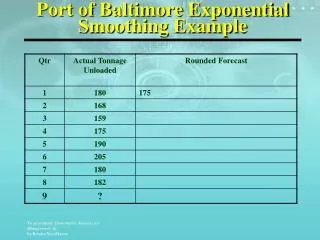
Application We will now forecastsales of liquor and floor covering using this technique. We have monthly data for each variable beginning in January 1999 and running through July of 2007.
Beer, Wine, Liquor = 0.1904Parts, Tires, etc. = 0.099 The ratio of the standard deviation to the mean gives us a nice measure of the amplitude or volatility of a series month-to-month (or day-to-day, quarter-to-quarter, as the case may be).
Selecting the smoothing constant • Pricey time series forecasting software, such as EViews, use an algorithm to select the value of the smoothing constant that minimizes mean square error for in-sample forecasts. • If you lack this software, you can use a trial and error process.
Forecasts for August, 2007 Remember our basic algorithm Hence to parts, accessories, and tire sales (PAT) for August, 2007: To forecast beer, wine, and liquor sales (BWL):