Download
1 / 48
490 likes | 1.24k Views
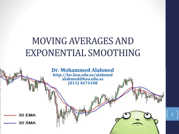
MOVING AVERAGES AND EXPONENTIAL SMOOTHING. Farideh Dehkordi-Vakil. Introduction. This chapter introduces models applicable to time series data with seasonal, trend, or both seasonal and trend component and stationary data. Forecasting methods discussed in this chapter can be classified as:

E N D
MOVING AVERAGES AND EXPONENTIAL SMOOTHING Farideh Dehkordi-Vakil
Introduction • This chapter introduces models applicable to time series data with seasonal, trend, or both seasonal and trend component and stationary data. • Forecasting methods discussed in this chapter can be classified as: • Averaging methods. • Equally weighted observations • Exponential Smoothing methods. • Unequal set of weights to past data, where the weights decay exponentially from the most recent to the most distant data points. • All methods in this group require that certain parameters to be defined. • These parameters (with values between 0 and 1) will determine the unequal weights to be applied to past data.
Introduction • Averaging methods • If a time series is generated by a constant process subject to random error, then mean is a useful statistic and can be used as a forecast for the next period. • Averaging methods are suitable for stationary time series data where the series is in equilibrium around a constant value ( the underlying mean) with a constant variance over time.
Introduction • Exponential smoothing methods • The simplest exponential smoothing method is the single smoothing (SES) method where only one parameter needs to be estimated • Holt’s method makes use of two different parameters and allows forecasting for series with trend. • Holt-Winters’ method involves three smoothing parameters to smooth the data, the trend, and the seasonal index.
Averaging Methods • The Mean • Uses the average of all the historical data as the forecast • When new data becomes available , the forecast for time t+2 is the new mean including the previously observed data plus this new observation. • This method is appropriate when there is no noticeable trend or seasonality.
Averaging Methods • The moving average for time period t is the mean of the “k” most recent observations. • The constant number k is specified at the outset. • The smaller the number k, the more weight is given to recent periods. • The greater the number k, the less weight is given to more recent periods.
Moving Averages • A large k is desirable when there are wide, infrequent fluctuations in the series. • A small k is most desirable when there are sudden shifts in the level of series. • For quarterly data, a four-quarter moving average, MA(4), eliminates or averages out seasonal effects.
Moving Averages • For monthly data, a 12-month moving average, MA(12), eliminate or averages out seasonal effect. • Equal weights are assigned to each observation used in the average. • Each new data point is included in the average as it becomes available, and the oldest data point is discarded.
Moving Averages • A moving average of order k, MA(k) is the value of k consecutive observations. • K is the number of terms in the moving average. • The moving average model does not handle trend or seasonality very well although it can do better than the total mean.
Example: Weekly Department Store Sales • The weekly sales figures (in millions of dollars) presented in the following table are used by a major department store to determine the need for temporary sales personnel.
Example: Weekly Department Store Sales • Use a three-week moving average (k=3) for the department store sales to forecast for the week 24 and 26. • The forecast error is
Example: Weekly Department Store Sales • The forecast for the week 26 is
Example: Weekly Department Store Sales • RMSE = 0.63
Exponential Smoothing Methods • This method provides an exponentially weighted moving average of all previously observed values. • Appropriate for data with no predictable upward or downward trend. • The aim is to estimate the current level and use it as a forecast of future value.
Simple Exponential Smoothing Method • Formally, the exponential smoothing equation is • forecast for the next period. • = smoothing constant. • yt = observed value of series in period t. • = old forecast for period t. • The forecast Ft+1 is based on weighting the most recent observation yt with a weight and weighting the most recent forecast Ft with a weight of 1-
Simple Exponential Smoothing Method • The implication of exponential smoothing can be better seen if the previous equation is expanded by replacing Ft with its components as follows:
Simple Exponential Smoothing Method • If this substitution process is repeated by replacing Ft-1 by its components, Ft-2 by its components, and so on the result is: • Therefore, Ft+1 is the weighted moving average of all past observations.
Simple Exponential Smoothing Method • The following table shows the weights assigned to past observations for = 0.2, 0.4, 0.6, 0.8, 0.9
Simple Exponential Smoothing Method • The exponential smoothing equation rewritten in the following form elucidate the role of weighting factor . • Exponential smoothing forecast is the old forecast plus an adjustment for the error that occurred in the last forecast.
Simple Exponential Smoothing Method • The value of smoothing constant must be between 0 and 1 • can not be equal to 0 or 1. • If stable predictions with smoothed random variation is desired then a small value of is desire. • If a rapid response to a real change in the pattern of observations is desired, a large value of is appropriate.
Simple Exponential Smoothing Method • To estimate , Forecasts are computed for equal to .1, .2, .3, …, .9 and the sum of squared forecast error is computed for each. • The value of with the smallest RMSE is chosen for use in producing the future forecasts.
Simple Exponential Smoothing Method • To start the algorithm, we need F1 because • Since F1 is not known, we can • Set the first estimate equal to the first observation. • Use the average of the first five or six observations for the initial smoothed value.
Example:University of Michigan Index of Consumer Sentiment • University of Michigan Index of Consumer Sentiment for January1995- December1996. • we want to forecast the University of Michigan Index of Consumer Sentiment using Simple Exponential Smoothing Method.
Example:University of Michigan Index of Consumer Sentiment • Since no forecast is available for the first period, we will set the first estimate equal to the first observation. • We try =0.3, and 0.6.
Example:University of Michigan Index of Consumer Sentiment • Note the first forecast is the first observed value. • The forecast for Feb. 95 (t = 2) and Mar. 95 (t = 3) are evaluated as follows:
Example:University of Michigan Index of Consumer Sentiment • RMSE =2.66 for = 0.6 • RMSE =2.96 for = 0.3
Holt’s Exponential smoothing • Holt’s two parameter exponential smoothing method is an extension of simple exponential smoothing. • It adds a growth factor (or trend factor) to the smoothing equation as a way of adjusting for the trend.
Holt’s Exponential smoothing • Three equations and two smoothing constants are used in the model. • The exponentially smoothed series or current level estimate. • The trend estimate. • Forecast p periods into the future.
Holt’s Exponential smoothing • Lt = Estimate of the level of the series at time t • = smoothing constant for the data. • yt = new observation or actual value of series in period t. • = smoothing constant for trend estimate • bt = estimate of the slope of the series at time t • m = periods to be forecast into the future.
Holt’s Exponential smoothing • The weight and can be selected subjectively or by minimizing a measure of forecast error such as RMSE. • Large weights result in more rapid changes in the component. • Small weights result in less rapid changes.
Holt’s Exponential smoothing • The initialization process for Holt’s linear exponential smoothing requires two estimates: • One to get the first smoothed value for L1 • The other to get the trend b1. • One alternative is to set L1 = y1 and
Example:Quarterly sales of saws for Acme tool company • The following table shows the sales of saws for the Acme tool Company. • These are quarterly sales From 1994 through 2000.
Example:Quarterly sales of saws for Acme tool company • Examination of the plot shows: • A non-stationary time series data. • Seasonal variation seems to exist. • Sales for the first and fourth quarter are larger than other quarters.
Example:Quarterly sales of saws for Acme tool company • The plot of the Acme data shows that there might be trending in the data therefore we will try Holt’s model to produce forecasts. • We need two initial values • The first smoothed value for L1 • The initial trend value b1. • We will use the first observation for the estimate of the smoothed value L1, and the initial trend value b1 = 0. • We will use = .3 and =.1.
Example:Quarterly sales of saws for Acme tool company • RMSE for this application is: = .3 and = .1 RMSE = 155.5 • The plot also showed the possibility of seasonal variation that needs to be investigated.
Winter’s Exponential Smoothing • Winter’s exponential smoothing model is the second extension of the basic Exponential smoothing model. • It is used for data that exhibit both trend and seasonality. • It is a three parameter model that is an extension of Holt’s method. • An additional equation adjusts the model for the seasonal component.
Winter’s Exponential Smoothing • The four equations necessary for Winter’s multiplicative method are: • The exponentially smoothed series: • The trend estimate: • The seasonality estimate:
Winter’s Exponential Smoothing • Forecast m period into the future: • Lt = level of series. • = smoothing constant for the data. • yt = new observation or actual value in period t. • = smoothing constant for trend estimate. • bt = trend estimate. • = smoothing constant for seasonality estimate. • St =seasonal component estimate. • m = Number of periods in the forecast lead period. • s = length of seasonality (number of periods in the season) • = forecast for m periods into the future.
Winter’s Exponential Smoothing • As with Holt’s linear exponential smoothing, the weights , , and can be selected subjectively or by minimizing a measure of forecast error such as RMSE. • As with all exponential smoothing methods, we need initial values for the components to start the algorithm. • To start the algorithm, the initial values for Lt, the trend bt, and the indices St must be set.
Winter’s Exponential Smoothing • To determine initial estimates of the seasonal indices we need to use at least one complete season's data (i.e. s periods).Therefore,we initialize trend and level at period s. • Initialize level as: • Initialize trend as • Initialize seasonal indices as:
Winter’s Exponential Smoothing • We will apply Winter’s method to Acme Tool company sales. The value for is .4, the value for is .1, and the value for is .3. • The smoothing constant smoothes the data to eliminate randomness. • The smoothing constant smoothes the trend in the data set.
Winter’s Exponential Smoothing • The smoothing constant smoothes the seasonality in the data. • The initial values for the smoothed series Lt, the trend Tt, and the seasonal index St must be set.
Example: Quarterly Sales of Saws for Acme tool • RMSE for this application is: = 0.4, = 0.1, = 0.3 and RMSE = 83.36 • Note the decrease in RMSE.
Additive Seasonality • The seasonal component in Holt-Winters’ method. • The basic equations for Holt’s Winters’ additive method are:
Additive Seasonality • The initial values for Ls and bs are identical to those for the multiplicative method. • To initialize the seasonal indices we use