Download
1 / 25
250 likes | 267 Views
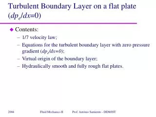
Turbulent Boundary Layer. Aerodynamics and Aeroelasticity Compressible Boundary layer.

E N D
Turbulent Boundary Layer Aerodynamics and Aeroelasticity Compressible Boundary layer
The phenomena observed during the transition process are similar for the flat plate boundary layer and for the plane channel flow, as shown in the following figure based on measurements by M. Nishioka et al. (1975). Periodic initial perturbations were generated in the BL using an oscillating cord. For typical commercial surfaces transition occurs at Re , 5x10⁵ However, the transition can be delayed to Re 3X10⁶by different ways such as having very smooth walls and/or very low turbulent wind tunnel.
The compressible boundary-layer for flow over a flat plate, where dpe/dx = 0 and steady state flow, these equations become Continuity X-momentum Y-momentum Energy
We note that the following: (1) the energy equation must be included, (2) the density is treated as a variable. (3) in general, μ and k are functions of temperature and hence also must be treated as variables. It is sometimes convenient to deal with total enthalpy, ho = h + V 2 /2, as the dependent variable in the energy equation, rather than the static enthalpy Note that, consistent with the boundary-layer approximation, where v is small, ho = h + V 2 /2 = h + (u + v2 )/2 ~ h + u2 / 2. (1)
we obtain (2) Recall that for a calorically perfect gas, dh = CpdT; hence, (3) Substituting last Equation into the above equation, we obtain (4)
We know And Replacing the above equations into (4). Finally, we obtain which is an alternate form of the boundary-layer energy equation. In this equation, Pris the local Prandtl number, which, in general, is a function of T and hence varíes throughout the boundary layer.
These are nonlinear partial differential equations. As in the incompressible case, let us seek a self-similar solution; however, the transformed independent variables must be defined differently: The dependent variables are transformed as follows: (which is consistent with defining stream function
Equations x.momemtum and (4) transform to (5) (6) They are ordinary differential equations- recall that the primes denote differentiation with respect to η. Therefore, the compressible, laminar flow over a flat plate does lend itself to a self-similar solution, where f' = f'(η) and g = g(η). That is, the velocity and total enthalpy profiles plotted versus ηare the same at any station. Furthermore, the product ρμ, is a variable and depends in part on temperature. Hence, we are dealing with a system of coupled ordinary differential equations which must be solved simultaneously.
The boundary conditions for these equations are Note that the coefficient u2/(ho)eappearing in Equation (4) is simply a function of the Mach number:
Therefore, equation (6) involves as a parameter the Mach number of the flow at the outer edge of the boundary layer, that is, for the flat-plate case, the free stream Mach number. Hence, we can explicitly see that the compressible boundary-layer solutions will depend on the Mach number. Moreover, because of the appearance of the local Pr in Equation (6) The solutions will also depend on the freestream Prandtlnumber as a parameter. Finally, note from the boundary conditions that the value of g at the wall gwis a given quantity. Note that at the wall where u = 0, gw= hw/(ho)e= cpTw/(ho)e.
Hence, instead of referring to a given enthalpy at the wall gw, we usually deal with a given wall temperature Tw. An alternative to a given value of Tw is the assumption of an adiabatic wall, that is, a case where there is no heat transfer to the wall. Then Since Equation (5) is third order, we need three boundary conditions at η= 0. We have only two, namely, Therefore, assume a value for and iterate until the boundary condition at the boundary-layer edge, f´= 1, is matched.
Similarly, Equation ( 6) is a second-order equation. It requires two boundary conditions at the wall in order to integrate numerically across the boundary layer; we have only one, namely, g(0) = gw· Thus, assume g'(0), and integrate Equation (6). Iterate until the outer boundary condition is satisfied; that is, g = 1. Since Equation ( 5) is coupled to Equation (6), that is, since ρμ, in Equation (5) requires a knowledge of the enthalpy ( or temperature) profile across the boundary layer, the entire process must be repeated again.
Typical solutions of Equations (5) and (6) for the velocity and temperature profiles through a compressible boundary layer on a flat plate are shown in next figures: Temperature profiles in a compressible laminar boundary layer over an insulated flat plate Velocity profiles in a compressible laminar boundary !ayerover an insulated flat plate
Both figures contain results for an insulated flat plate (zero-heat transfer) using Sutherland's law for μ,, and assuming a constant Pr = 0.75. The velocity profiles are shown for different Mach numbers ranging from 0 (incompressible flow) to the large hypersonic value of 20. Note that at a given x station a ta given Rex . the boundary layer thickness increases markedly as Me is increased to hypersonic values. This clearly demonstrates one of the most important aspects of compressible boundary layers, namely, that the boundary-layer thickness becomes large at large Mach numbers. Temperature figure illustrates the temperature profiles for the same case. Note the obvious physical trend that, as Me increases to large hypersonic values, the temperatures increase markedly Also note that at the wall as it should be for an insulated surface (qw= 0).
Temperature profiles in a laminar, compressible boundary layer over a cold flat plate Velocity profiles in a laminar, compressible boundary layer over a cold flat plate.
This illustrates the general fact that the effect of a cold wall is to reduce the boundary-layer thickness. This trend is easily explainable on a physical basis when we examine the temperature profile figure. Comparing, temperature profile figures for insulated and cold plate, we note that, as expected, the temperature levels in the cold-wall case are considerably lower than in the insulated case. Because the pressure is the same in both cases, we have from the equation of state p = ρRT, that the density in the cold-wall case is much higher. If the density is higher, the mass flow within the boundary layer can be accommodated within a smaller boundary-layer thickness; hence, the effect of a cold wall is to thin the boundary layer.
Noting on the temperature profile of cold plate figure, starting at the outer edge of the boundary layer and going toward the wall, the temperature first increases, reaches a peak somewhere within the boundary layer, and then decreases to its prescribed cold-wall value of Tw. The peak temperature inside the boundary layer is an indication of the amount of viscous dissipation occurring within the boundary layer.
REYNOLDS ANALOGY Reynolds analogy is a relation between the skin friction coefficient and the heat transfer coefficient. we define the skin friction coefficient as for Couette flow, Combining both equations Then
REYNOLDS ANALOGY It demonstrates that the skin friction coefficient is a function of just the Reynolds number-a result which applies in general for other incompressible viscous flows Now let us define a heat transfer coefficient as CH is called the Stanton number; it is one of several! Different types of heat transfer coefficient that is used in the analysis of aerodynamic heating. For Couetteflow and
REYNOLDS ANALOGY we have for Couetteflow we obtain We now combine the results for Cfand CH obtained above.
REYNOLDS ANALOGY In tum, the surface values Cfand CH can be obtained from the velocity and temperature gradients respectively at the wall as given by the velocity and temperature profiles evaluated at the wall. where (∂u/∂y)w and (∂T /∂y)w are the values obtained from the velocity and temperature profiles, respectively, evaluated at the wall. In turn, the overall flat plate skin friction drag coefficient Cfcan be obtained by integrating cfover the plate via
REYNOLDS ANALOGY From this equation For the friction drag coefficient for incompressible flow The analogous compressible result can be written as for the thickness of the incompressible flat-plate boundary layer. The analogous result for compressible flow is
REYNOLDS ANALOGY Friction drag coefficient for laminar, compressible flow over a flat plate, illustrating the effect of Mach number and wall temperature. Pr = 0.75.
REYNOLDS ANALOGY Boundary-layer thickness for laminar, compressible flow over a flat plate, illustrating the effect of Mach number and wall temperature. Pr = 0.75.
REYNOLDS ANALOGY A directly analogous result holds for the compressible fiat-plate flow. If we assume that the Prandtl number is constant, then for a flat plate, Reynolds analogy is, from the numerical solution, The local skin friction coefficient cf for the incompressible flat-plate case, becomes the following form for the compressible flat-plate flow: