Download

1 / 22
250 likes | 532 Views
Selected Hyperspectral Mapping Method. Mirza Muhammad Waqar Contact: mirza.waqar@ist.edu.pk +92-21-34650765-79 EXT:2257. RG712. Course: Special Topics in Remote Sensing & GIS. Outlines . Hyperspectral Data Hyperspectral vs Multispectral Data Analysis Hyperspectral Mapping Techniques

E N D
Selected Hyperspectral Mapping Method Mirza Muhammad Waqar Contact: mirza.waqar@ist.edu.pk +92-21-34650765-79 EXT:2257 RG712 Course: Special Topics in Remote Sensing & GIS
Outlines • Hyperspectral Data • Hyperspectral vs Multispectral Data Analysis • Hyperspectral Mapping Techniques • Spectral Angle Mapper • Matched Matching • Spectral Feature Fitting • Binary Encoding (BE) • Complete Linear Spectral Unmixing • Match Filtering
Revision – Hyperspectral Thematic Mapping • Imaging Spectrometry • Multispectral versus Hyperspectral • Hyperspectral Image Acquisition • Extraction of information from Hyperspectral data • Preprocessing of Data • Subset Study Area • Initial Image Quality Assessment • Visual Individual Band Examination • Visual Examination of Color Composite • Animation • Statistical Individual Band Examination • Radiometric Calibration • In situ data • Radiosounder • Radiative Transfer based Atmospheric Correction DN Value Radiance Irradiance Apparent Reflectance (Albedo) Reflectance
Revision – Hyperspectral Thematic Mapping • Selected Atmospheric Correction Models • Flat Field Correction • Internal Average Relative Reflectance (IARR) • Empirical Line Calibration • Reducing Data Redundancy • Principal Component Transformation • Minimum Noise Fraction Transformation (MNF) • Endmember Determination • Pixel Purity Index (PPI) • n-dimensional visualization of endmembers in feature space • Hyperspectral Mapping Method • Spectral Angle Mapper (SAM)
Hyperspectral Data • In order to be considered a specific data as hyperspectral, three conditions should be satisfied. • Multiple bands • High spectral resolution (i.e. narrowness of each band) • Contiguity of bands. • Landsat • ASTER • MODIS • AVIRIS • Hyperion
Multispectral vs Hyperspectral Mapping • Multispectral Analysis methods are generally inadequate when applied to hyperspectral data: • Inefficient: • Multispectral methods are too computationally intensive when applied to high dimensional data • Accuracy degradation • Classification accuracy can actually decrease with the addition of extra bands that do not contribute meaningful information content. • Loss of subtle detail • The standard multispectral pattern recognition methods ultimately equate variance with information, which often results in subtle spectral variations being lost in the noise.
Hyperspectral Mapping Techniques • Atmospheric Correction • Classification and target identification • Whole pixel method • Spectral Angle Mapper • Spectral Feature Fitting • Subpixel method • Complete Linear Spectral Unmixing • Matched Filtering • Others • Neural network • Decision boundary feature extraction (DBFE)
Spectral Angle Mapper (SAM) • SAM compares test image spectra to a known reference spectra using the spectral angle between them. • This method is not sensitive to illumination since the SAM algorithm uses only the vector direction and not the vector length. a = spectral angle between two spectra n = number of bands Ti = reflectance value of band i in the test spectra Ri = reflectance value of band i in the reference spectra
Continuum Removal A continuum is a mathematical function used to isolate a particular absorption feature for analysis (Clark and Roush, 1984; Kruse et al, 1985; Green and Craig, 1985). LC= Continuum Removed Spectra using library spectra L = Library Spectra Cλ = Least Square fit factor
Matched Matching • Spectral Feature Fitting (SFF): A least-squares technique. SFF is an absorption-feature-based methodology. The reference spectra are scaled to match the image spectra after continuum removal from both data sets. (e.g. Tetracorder) • Examines absorption features • Depth • Shape • Ex. Tetracorder by USGS • http://speclab.cr.usgs.gov/tetracorder.html
Spectral Feature Fitting (SFF) • Where • Rb is reflectance in band center • Rc is reflectance in continuum at band center Use specific bands to search for individual features and estimate a relative concentration based on band depth. First generate a continuum-removed spectrum for a specific feature in order to compare it with library spectra and image-derived spectra. Convolve library spectra with spectral response of sensor to generate an estimate of image derived reflectance spectra (i.e., assumes some form of atmospheric inversion has been applied to image data).
Matched Matching • Binary Encoding (BE): The binary encoding classification technique encodes the data and end member spectra into 0s and 1s based on whether a band falls below or above the spectrum mean. An exclusive OR function is used to compare each encoded reference spectrum with the encoded data spectra and a classification image produced.
Binary Encoding (BE) • Compute spectral mean of a sample (pixel) • Assign a 1 to bands equal or greater than mean and 0 to those less than mean. • Do the same for reference (e.g. spectral library) spectra. • Compare the pattern as a measure of similarity. • Compute spectral mean Rm of sample (pixel) over a local waveband of interest • Assign a 1 to bands equal or greater than mean and 0 to those less than mean: • If R(λ) ≥ Rm assign a “1” • If R(λ) < Rm assign a “0”
Linear vs Non-Linear Mixing Linear Mixing
Complete Linear Spectral Unmixing • Calculate the fractions of endmembers in each pixel • Endmembers • Spectrally unique surface materials • Similar to fuzzy classification with multispectral data analysis • Results • An abundance image, and • Membership images
Matched Filtering • Partial unmixing technique • Originally developed to compute abundances of targets that are relatively rare in the scene. • Matched Filtering “filters” the input image for good matches to the chosen target spectrum by maximizing the response of the target spectrum within the data and suppressing the response of everything else. • One potential problem with Matched Filtering is that it is possible to end up with false positive results.
Hyperspectral Data Acquisition Raw Radiance Data Spectral Calibration At-Sensor Spectrally Calibrated Radiance Spatial Pre-Processing and Geocoding Radiometrically and Spatially processed radiance image Atmospheric Correction, solar irradiance correction Geocoding reflectance image Feature Mapping Data analysis for feature mapping Absorption band characterization Spectral feature fitting Spectral Angle Mapping Spectral Unmixing Minral Maps