Nowcasting of thunderstorms

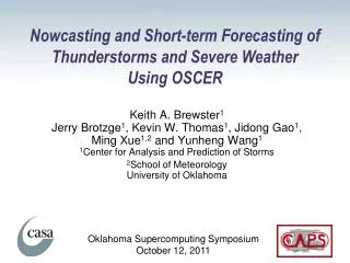
1. Nowcasting of thunderstorms Valliappa.Lakshmanan@noaa.gov National Severe Storms Laboratory & University of Oklahoma Seminar at City University of New York CREST program http://cimms.ou.edu/~lakshman/ Valliappa.Lakshmanan@noaa.gov

2. What is nowcasting? • Skilled short-term estimates and predictions • Typically 0-60 minutes • For emergency managers, transportation, etc. • Made by meteorologists • With guidance from automated algorithms • Guidance to forecasters involves supplying estimates & predictions for: • Spatial location of thunderstorms • Where is the storm now? What is the path the storm has traveled? • Where will the storm be in 30 minutes? • Intensity of thunderstorms • Weakening? Strengthening? • Potential hazards • Hail? Lightning? Tornadoes? Flooding? Valliappa.Lakshmanan@noaa.gov

3. Hazard prediction • This talk will focus on estimating and predicting: • Spatial location of thunderstorms • Intensity characteristics of thunderstorms • Hazard prediction is carried out by tailored algorithms • Hail Detection Algorithm • Looks for high radar reflectivity aloft • Cores may descend to cause hail • Flash flood prediction algorithm • Estimate rainfall amount based on radar reflectivity • Accumulate rainfall in delineated basins • Couple with flow model (soil moisture, etc.) • Etc. Valliappa.Lakshmanan@noaa.gov

4. How to do nowcasting • Numerical models • Can not be done in real-time • Skill of numerical models an area of much research • May be the future • Rule-based prediction of growth and decay • Identify boundaries from multiple sensors or human input • Extrapolate echoes likely to persist or form • Approach of “Auto Nowcaster” from NCAR • Qualitatively: works • Quantitatively: similar issues as numerical models • Linear extrapolation of radar echoes • Highly skilled in the short term (under 60 minutes) • Can be done in real-time • Assumption is of steady-state (no growth/decay) Valliappa.Lakshmanan@noaa.gov

5. Methods for estimating movement • Linear extrapolation involves: • Estimating movement • Extrapolating based on movement • Techniques: • Object identification and tracking • Find cells and track them • Optical flow techniques • Find optimal motion between rectangular subgrids at different times • Hybrid technique • Find cells and find optimal motion between cell and previous image Valliappa.Lakshmanan@noaa.gov

6. Some object-based methods • Storm cell identification and tracking (SCIT) • Developed at NSSL, now operational on NEXRAD • Allows trends of thunderstorm properties • Johnson J. T., P. L. MacKeen, A. Witt, E. D. Mitchell, G. J. Stumpf, M. D. Eilts, and K. W. Thomas, 1998: The Storm Cell Identification and Tracking Algorithm: An enhanced WSR-88D algorithm. Weather & Forecasting, 13, 263–276. • Multi-radar version part of WDSS-II • Thunderstorm Identification, Tracking, Analysis, and Nowcasting (TITAN) • Developed at NCAR, part of Autonowcaster • Dixon M. J., and G. Weiner, 1993: TITAN: Thunderstorm Identification, Tracking, Analysis, and Nowcasting—A radar-based methodology. J. Atmos. Oceanic Technol., 10, 785–797 • Optimization procedure to associate cells from successive time periods • Satellite-based MCS-tracking methods • Association is based on overlap between MCS at different times • Morel C. and S. Senesi, 2002: A climatology of mesoscale convective systems over Europe using satellite infrared imagery. I: Methodology. Q. J. Royal Meteo. Soc., 128, 1953-1971 • http://www.ssec.wisc.edu/~rabin/hpcc/storm_tracker.html • MCSs are large, so overlap-based methods work well Valliappa.Lakshmanan@noaa.gov

7. Object-based methods, pros & cons • How object-based methods work: • Identify high-intensity clump of pixels as “cells” • Associate cells between time frames • Closest distance/values/overlap, etc. • Pros: • Small-scale prediction • Can find out history of a thunderstorm (“trends”) • Cons: • Splits and merges hard to keep track of • Hard to avoid association errors • Most storm cells last only about 20 minutes • Large-scale predictions are difficult to build up Valliappa.Lakshmanan@noaa.gov

8. Optical flow methods • How optical flow methods work • Take rectangular region around each pixel of current image • Move rectangular window around previous image • Choose movement that minimizes error between images • Need to ensure that successive pixels do not have very different movements • Do not identify and associate cells • Pro: Removes cell identification and association errors • Con: No trends possible • Not affected by splits/merges • Pro: More accurate motion estimates • Con: Small-scale tracking not possible • Poor motion estimates where no storms available in current/previous image • Often have to use global movement • Or interpolate between storms Valliappa.Lakshmanan@noaa.gov

9. Some optical flow methods • TREC • Minimize mean square error within subgrids between images • No global motion vector, so can be used in hurricane tracking • Results in a very chaotic wind field in other situations • Tuttle, J., and R. Gall, 1999: A single-radar technique for estimating the winds in tropical cyclones. Bull. Amer. Meteor. Soc., 80, 653-668 • Large-scale “growth and decay” tracker • MIT/Lincoln Lab, used in airport weather tracking • Smooth the images with large elliptical filter, limit deviation from global vector • Not usable at small scales or for hurricanes • Wolfson, M. M., Forman, B. E., Hallowell, R. G., and M. P. Moore (1999): The Growth and Decay Storm Tracker, 8th Conference on Aviation, Range, and Aerospace Meteorology, Dallas, TX, p58-62 • McGill Algorithm of Precipitation by Lagrangian Extrapolation (MAPLE) • Variational optimization instead of a global motion vector • Tracking for large scales only, but permits hurricanes and smooth fields • Germann, U. and I. Zawadski, 2002: Scale-dependence of the predictability of precipitation from continental radar images. Part I: Description of methodology. Mon. Wea. Rev., 130, 2859-2873 Valliappa.Lakshmanan@noaa.gov

10. Need for hybrid technique • Need an algorithm that is capable of • Tracking multiple scales: from storm cells to squall lines • Storm cells possible with SCIT (object-identification method) • Squall lines possible with LL tracker (elliptical filters + optical flow) • Providing trend information • Surveys indicate: most useful guidance information provided by SCIT • Estimating movement accurately • Like MAPLE • How? Valliappa.Lakshmanan@noaa.gov

11. Technique • Identify storm cells based on reflectivity and its “texture” • Merge storm cells into larger scale entities • Estimate storm motion for each entity by comparing the entity with the previous image’s pixels • Interpolate spatially between the entities • Smooth motion estimates in time • Use motion vectors to make forecasts Courtesy: Yang et. al (2006) Valliappa.Lakshmanan@noaa.gov

12. Why it works • Hierarchical clustering sidesteps problems inherent in object-identification and optical-flow based methods Valliappa.Lakshmanan@noaa.gov

13. Advantages of technique • Identify storms at multiple scales • Hierarchical texture segmentation using K-Means clustering • Yields nested partitions (storm cells inside squall lines) • No storm-cell association errors • Use optical flow to estimate motion • Increased accuracy • Instead of rectangular sub-grids, minimize error within storm cell • Single movement for each cell • Chaotic windfields avoided • No global vector • Cressman interpolation between cells to fill out areas spatially • Kalman filter at each pixel to smooth out estimates temporally Valliappa.Lakshmanan@noaa.gov

14. 1. Identifying storms: K-Means clustering • Obtain a vector of measurements at each pixel • Statistics in neighborhood of each pixel (called “texture”) • Can also use multiple sensors or channels • Divide up vector space into K “bands” • The bands can be equally spaced by equal-probability • Center the clustering algorithm at each of these bands • Assign each pixel to the band that it lies in • Perform region growing • Pixels in same band adjacent to each other are part of region • Compute region properties • Move pixel from one region to another if cost function lowered • Cost function lower if pixel moves to region whose mean texture it is closer to • Cost function lower if pixel moves to region that it is closer (spatially) to • Iterate until stable Valliappa.Lakshmanan@noaa.gov

15. The cost function • The cost function takes into account • Textural similarity between pixel at x,y and the mean texture of kth cluster • Spatial contiguity of pixel to cluster • Weighted appropriately (lambda=0.2 seems to work well) Valliappa.Lakshmanan@noaa.gov

16. Radar reflectivity K=4 clustering Clustering: example Valliappa.Lakshmanan@noaa.gov

17. 2. Hierarchical clustering • At the end of iteration, all pixels have been assigned to their best clusters • Most detailed scale of segmentation • Scale=0 • Clusters are typically very small • Combine clusters to form larger regions • Find mean inter-cluster distance • Combine regions which are spatially adjacent whose textural means are close to each other • Repeat to get largest regions Reflectivity Scale=0 Scale=1 Scale=2 Valliappa.Lakshmanan@noaa.gov

18. 3. Compute motion estimates • Starting with scale=2, project the current cluster backward • Move the cluster around within the previous image • Choose the movement that minimizes mean absolute error • Minimization based on kernel estimate, to reduce outlier errors • A motion estimate obtained for each cluster • Less noisy than pixel-based estimates • Automatic smoothing over region of cluster • Scale=0 is the noisiest (fewer pixels) • What about newly developing cells? • Limit the search space to maximum expected storm movement • If mean absolute error is too large, assume that cell is new • Will take movement based on neighboring cells Valliappa.Lakshmanan@noaa.gov

19. 4. Spatially interpolate motion vectors • Need motion estimate between regions • Spatially interpolate between regions • Weighted by distance from region (Cressman weights) • Weighted by size of region • Fill out spatial grid • Can use background wind field to fill out domain • Constant weight for background wind field (from model) • Use scale=2 motion estimate as background field for scale=1 • Repeat process to get motion vector for scale=2 • Use scale=1 motion estimate as background field for scale=0 • Repeat process to get motion vector for scale=1 Valliappa.Lakshmanan@noaa.gov

20. 5. Kalman filter • Motion estimates are smoothed in time • Each pixel runs a Kalman filter (constant acceleration model) • Smoothes the motion estimates Courtesy: Yang et. al (2006) Valliappa.Lakshmanan@noaa.gov

21. 6. Use motion estimate to do forecast • Forward • Using motion estimate at a pixel, project the point to where it should be • Create a spatial Gaussian distribution of the point’s value at that location • Interpolation • For fast moving storms, it is possible that there will be gaps in the output field • Interpolate between projected points • Use different scales for different time periods, for example: • Use scale=0 for forecasting less than 15 minutes • Use scale=1 for forecasting 15-45 minutes • Use scale=2 for forecasting longer than 45 minutes Valliappa.Lakshmanan@noaa.gov

22. 7. Trends • What about trends? • Compute properties of current cluster • Min, max, mean, count, histogram, etc. • Project cluster backwards onto previous sets of images • Can use fields other than the field being tracked • Compute properties of projected cluster • Use to diagnose trends • Not used operationally yet Valliappa.Lakshmanan@noaa.gov

23. Example: hurricane (Sep. 18, 2003) Image Scale=1 Eastward s.ward Valliappa.Lakshmanan@noaa.gov

24. Satellite water vapor (Feb. 28, 2003) Image 30-min forecast 60-min forecast Valliappa.Lakshmanan@noaa.gov

25. Typhoon Nari (Taiwan, Sep. 16, 2001) • Composite reflectivity and CSI for forecasts > 20 dBZ • Large-scale (temporally and spatially) Courtesy: Yang et. al (2006) Valliappa.Lakshmanan@noaa.gov

26. Complete life-cycle of a storm: CSI at different scales and time periods Tornado case (Apr. 20, 1995) Valliappa.Lakshmanan@noaa.gov

27. Tornado case (May 8, 2003) Courtesy: Yang et. al (2006) Valliappa.Lakshmanan@noaa.gov

28. Comparison with other techniques (dBZ)KTLX, May 3 1999 Bias CSI • Forecasting reflectivity through different techniques (30min) • Persistence • TREC (xcorr) • Same wind-field for all storms • Hierarchical K-Means + Kalman MAE Valliappa.Lakshmanan@noaa.gov

29. Comparison with other techniques (VIL) KTLX, May 3 1999 Bias CSI • Forecasting VIL through different techniques (30 min) • Persistence • TREC (xcorr) • Same wind-field for all storms • Hierarchical K-Means + Kalman MAE Valliappa.Lakshmanan@noaa.gov

30. Forecast loop of VIL (May 3, 1999) Valliappa.Lakshmanan@noaa.gov

31. References • Technique described in this paper: • Lakshmanan, V., R. Rabin, and V. DeBrunner, 2003: Multiscale storm identification and forecast. J. Atm. Res., 67-68, 367-380 • http://cimms.ou.edu/~lakshman/Papers/kmeans_motion.pdf • Some of the results shown here are from: • Yang, H., J. Zhang, C. Langston, S. Wang (2006): Synchronization of Multiple Radar Observations in 3-D Radar Mosaic, 12th Conf. on Aviation, Range and Aerospace Meteo. Atlanta, GA, P1.10 • http://ams.confex.com/ams/pdfpapers/104386.pdf • Software implementation • w2segmotion is one of the algorithms that is part of WDSS-II • Lakshmanan, V., T. Smith, G. J. Stumpf, and K. Hondl, 2006 (In Press): The warning decision support system - integrated information (WDSS-II). Weather and Forecasting. • http://www.wdssii.org/ Valliappa.Lakshmanan@noaa.gov