Download
1 / 40
431 likes | 714 Views
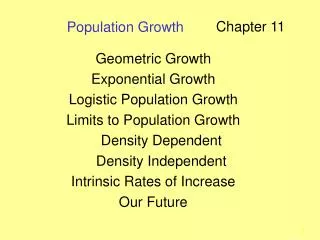
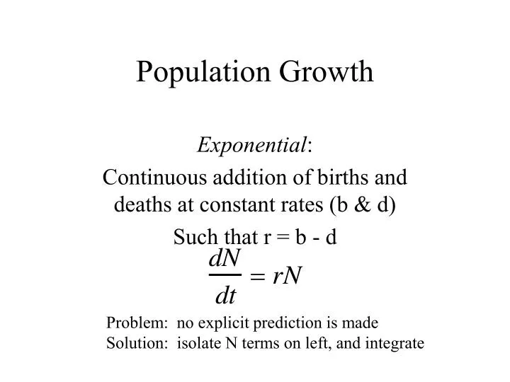
Population Growth. Exponential : Continuous addition of births and deaths at constant rates (b & d) Such that r = b - d. Problem: no explicit prediction is made Solution: isolate N terms on left, and integrate. Result of the integration:. r=0.05. Exponential growth relationships.

E N D
Population Growth Exponential: Continuous addition of births and deaths at constant rates (b & d) Such that r = b - d Problem: no explicit prediction is made Solution: isolate N terms on left, and integrate
Result of the integration: r=0.05
Exponential growth relationships Slope of Curve on left Density Slope of this curve Increases with density Slope of line = r
Exponential growth, log scale Linear increase of log values with time is a sign of exponential growth
Geometric Growth Time is measured in discrete (contant) chunks Simplest approach: Generations are the time unit R0: Average number of offspring produced per individual, per lifetime-- Factor that a population will be multiplied by for each generation. Often called the Net Rate of Increase. Time is measured in generations in this equation.
Relationship between R0 and r A population growing for one generation should show the same result using either of the following equations: Discrete, where T=1 generation Continuous, where t=t (t = “generation time”) If these give the same result, then
R0 and r So! Information about R and t can lead us to r
Assumptions of exponential or geometric growth projections Constant lx and mx schedules This implies that reproduction and survival will not change with density This also implies that any changes in physical or chemical environment have no influence on survival or reproduction No important interactions with other species if age-specific data are used, assume stable age distribution.
Suppose we let lx, mx and t vary with density Bottom line: let r (per capita growth rate) vary with N r dN/Ndt 0 0 K N
Density-dependent growth r dN/Ndt -r/K 0 0 N K Y = A + BX
Logistic equation Predictive form:
Logistic Examples Full-loop (2x the bacteria) Half-loop (half that on right) Paramecium, 2 species, growing for 8 days at high <r> and low <l> resource levels. Scale has been stretched on right to be equivalent to that on the left
More logistic examples Growth of flour beetles in flower, In containers holding different amts of flour Growth of a zooplankton crust- acean, Moina, at different temperatures
Evolution of K in Drosophila Post-radiation Hybrid Inbred Control Results suggest that K responds to an increase in genetic variation, And that it changes gradually through time in response to selection.
Assumptions of Logistic Growth Constant environment (r and K are constants) Linear response of per capita growth rate to density Equal impact of all individuals on resources Instantaneous adjustment of population growth to change in N No interactions with species other than those that are food Constantly renewed supply of food in a constant quantity
Discrete Model for Limited Growth Same assumptions, except population grows in bursts with each Generation-- built-in time lag Models of this sort show the potential influence that a time lag can have on population change.
Simple model, complex behavior R = 0.1, K = 1000
Simple model, complex behavior R = 1.9, K = 1000 Damped oscillation
Simple model, complex behavior r= 2.2, K = 1000 Limit cycle
Simple model, complex behavior r= 2.5, K = 1000 4-point cycle
Simple model, complex behavior r= 2.58, K = 1000 8-point cycle
Simple model, complex behavior r= 2.7, K = 1000 Erratic
Chaos r= 3, K = 1000
Overshoot, Crash, Extinction r= 3.000072, K = 1000
Concerns about Chaos Biological populations don’t appear to have the growth capacity to generate chaos, but this shows the potential importance of time lags. More complicated models can be even more sensitive Some systems might be completely unpredictable
Evolution of Life Histories Life history features: Rates of birth, death, population growth Patterns of reproduction and mortality Behavior associated with reproduction Efficiency of resource use, and carrying capacity Anything that affects population growth