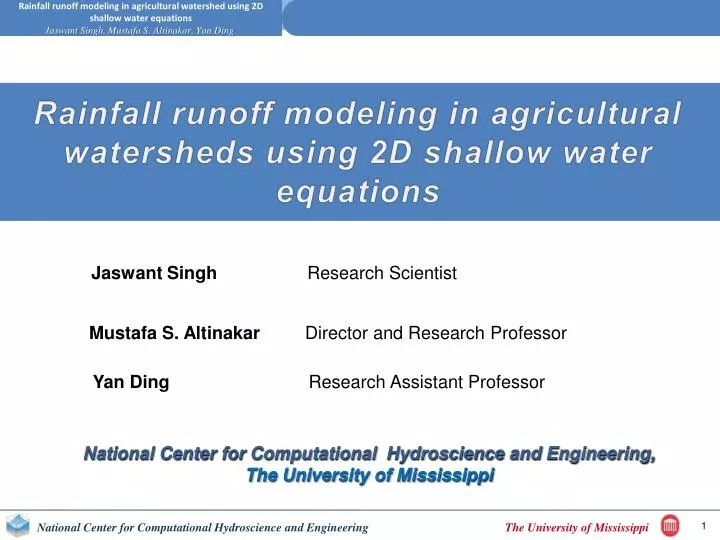
Rainfall runoff modeling in agricultural watersheds using 2D shallow water equations

1. Rainfall runoff modeling in agricultural watersheds using 2D shallow water equations Jaswant Singh Research Scientist Mustafa S. AltinakarDirector and Research Professor Yan Ding Research Assistant Professor National Center for Computational Hydroscience and Engineering, The University of Mississippi

2. Outline • Outline • Motivation and significance • Model development, solution scheme description. • Validation with analytical, laboratory and field experimental results. • Application: • Goodwin Creek watershed • Conclusions

3. Motivation and Significance • MOTIVATION & SIGINIFICANCE • Heavy storm events can trigger devastating floods. • Loss of life • Queensland, Australia, Jan.10th, 2011, 35 dead and 9 missing (Bloomberg Business week (209.45 MM 24 hour rainfall)Bombay India July 26th, 2005, 1097 people dead reason catastrophic rain.(24-hours rainfall 994 mm (39.1 inch) • France (Dec, 2, 1959, Malpasset dam break due to catastrophic rainfall event killing 421 (Wikipedia) • Property loss (billions of dollars) • Infrastructure loss • Agricultural damage (billions of dollars)

4. Motivation and Significance • MOTIVATION & SIGINIFICANCE • Flash floods: • Overland flow which results from rains (rainfall chraterisitcs), antecedent moisture conditions, terrain slope and soil properties of the terrain. • Solutions: • Rainfall- runoff modeling (SWAT, AnnAGNPS and hydrological models) • Advantage: Fast and covers large domains. • Disadvantage: (Inundation map, velocities, flood arrival time, water depths at any point in the flood plain is not possible). Only hydrograph at the outlet of the watershed is possible.

5. Motivation and Significance • Literature Review • Feature of the present model: • Chow and Ben-Zvi 1973;Hromadka et al. 10987, Zhang and Cundy 1989, Tyafur et al. 1993) have limited their applications to constant rainfall intensity and spatially constant infiltration rate. • Costabile et al.2011 presented a comparative analysis of overland flow models and found that in test cases where the bottom topography is complicated, only dynamic models (SWE based) could produce good results for discharge and water depths. • This models considers spatial and temporal variability of rainfall with multiple rain gauges. • Spatial variability of infiltration rates. • Second order accurate, positivity preserving solution scheme

6. Motivation and Significance • Objectives • To develop an overland model with the following features: • Inundation map, water surface elevation, water depth, discharge, velocity, flood arrival time at any cell in the flood plain. • Spatial and temporal variation simple as well as compound rainfall events recorded by multiple rain gauge. • Spatial variation of soil properties and landuse. Hence spatially varying infiltration. • Robust and easy to implement. • Easy to parallelize for fast computations using GPUs.

7. Model Development (SWE) 2D Shallow Water Equations (SWE) in vector notation Friction terms in X, Y direction R=Rainfall Intensity I=Infiltration Rate Bottom elevation terms in X,Y direction Vector of conserved variables Vector of fluxes in x direction Vector of fluxes in y direction Source and sink terms

8. Model Development (Solution Scheme description) Varibale definitions Rain R(x,y,t) h B w Front view of the domain w,u,v (nodes) Infiltration (I) B (nodes) Computational Grid B is bilinearily interpolated at the center of the cell

9. Model Development (Kurganov & Petrova 2007) H= Numerical flux of w, hu, hv in x and y direction a = local speed of wave propagation in X direction

10. Model Development (Source and sink Terms treatment) Treatment of source and sink terms Momentum: Bottom gradient and friction terms C= Chezy’s coefficient N= manning coefficient

11. Model Development (Source and sink Terms treatment) Rainfall source terms • Rainfall: R(x,y,t) Rainfall Intensity (mm/hr) • Rain gauge: Multiple location (spatial and temporal variability of rainfall • Average rainfall: Least distance method for assigning the cells to the nearest rain gauge

12. R(x,y,t) θ h0 Ponded water Saturated zone L Wetting front θi Δθ Unsaturated zone η θe θr Z Infiltration variables definition in the Green Ampt method variables Model Development (Source and sink Terms treatment) Infiltration Rate (mm/hr) • Green and Ampt method (1911) Rainfall intensity (mm/hr) Green and Ampt method parameters L: Depth of the wetting zone η: Porosity Ks: Saturated hydraulic conductivity θi: Initial moisture content of the soil Δθ : (θs - θi) θr : Residual moisture content of the soil after thoroughly drained. θs: Saturated moisture content Ψ =wetting front dry suction head, This method is based on Darcy’s law.93

13. Model Development (Source and sink Terms treatment) Infiltration Capacity (mm/hr) • Green and Ampt method (1911) Ψ = dry suction head F = total infiltration in time t Discretizing using Euler’s method Green and Ampt Method parameters: Porosity (n), Saturated moisture content (θs), wetting front dry suction head (Ψ), hydraulic conductivity (Ks), θe effective porosity, Se= Effective saturation (0-1)

14. Validation with analytical results Analytical test results Gottardi and Venutelli (1993) AWR Domain = 500m X 400m Impervious bottom Slope (x)=0.0005 Slope (y) =0.0 R= 0.33mm/min, constant in time n= 0.02 m-1/3s ∆x = ∆y = 0.05m. Outlet = cell (1 x 1) Reasonably good match with analytical results

15. Validation with field experiments Rainfall-Runoff Field experiment Peugeot et. al. 1997 Niger (South Africa) Total plot area =71.25 m2 Grid spacing = 0.25m R= Rainfall intensity (temporally varying storm) n= 0.02 m-1/3s Outlet = downstream side (complete side) Storm simulated =4 Average slope X direction =0.0196 Average slope Y direction =0.064 Surface profile of the experimental field at Niger, West Africa.

16. Simulation Results)

17. Simulation Results) Comparison of simulated runoff with field observed runoff for storm dated August 10, 1994 (calibration run).

18. Simulation Results) Comparison of simulated runoff with field observed runoff for storm dated August 7, 1994.

19. Simulation Results) Simulated water depth, velocity vectors over the experimental field at 750 seconds for the storm dated August 25, 1994.

20. Simulation Results) Animation of overland flow with velocity vectors for storm 3

21. Simulation Results) Comparison of simulated runoff with field observed runoff for storm dated September 4, 1994

22. Application: Goodwin Creek Watershed Rainfall-Runoff modeling at Goodwin Creek Watershed Total area in DEM = 55 Km2 , Watershed area=21.3 Km2 No. of Cells in the DEM =307 X202, Grid size= 30 meters No. of Rain Gauge Station=31 Solution Method= KP Model Infiltration method = Green and Ampt method. Infiltration parameters =Spatially variable Manning’s = Spatially variable Storm 1 Date =17-18, october-1981 2 Date= January 20th, 21th, 22nd and 23rd, 1982

23. Application: Goodwin Creek Watershed Rainfall-Runoff modeling at Goodwin Creek Watershed Rain Gauge Stations

24. Application: Goodwin Creek Watershed Rainfall-Runoff modeling at Goodwin Creek Watershed

25. Calibration of parameters: Goodwin Creek watershed Rainfall-Runoff modeling at Goodwin Creek Watershed Calibrated parameters for Green and Ampt method and Manning’s n for Goodwin creek soils and landuse

26. Application: Goodwin Creek Watershed Rainfall-Runoff modeling at Goodwin Creek Watershed Comparison of simulated and field observed runoff on 17th and 18th October 1981

27. Application: Goodwin Creek Watershed Rainfall-Runoff modeling at Goodwin Creek Watershed Comparison of simulated and field observed runoff on January 20th, 21th, 22nd and 23rd, 1982

28. Application: Goodwin Creek Watershed Rainfall-Runoff modeling at Goodwin Creek Watershed Overland flow depth (m) Velocity vectors Various maps at 15.9 hours for storm no. 2 in Goodwin creek watershed Wetting front depth (m)

29. Conclusions • A 2D numerical model is developed using Kurganov and Petrova 2007 scheme for simulation of flush floods. • The scheme is well balanced, robust and positivity preserving. • The model is tested against the field level experimental data and found that the simulated results match well with the experimental result for runoff at the outlet of the field. • The model is applied in real life case of Goodwin Creek watershed. • Spatial and temporal variability of rainfall and spatial variability of soil properties and landuse is incorporated in the model. • Two storm events simulated by the model match well with the observations at the watershed outlet

30. Acknowledgements This research was funded by the Department of Homeland Security-sponsored Southeast Region Research Initiative (SERRI) at the Department of Energy’s Oak Ridge National Laboratory, USA.

31. Simulation Results) Eq. 1 Flux computations Eq. 2 Eq. 3

32. Eq. 4 Subtracting Bij from both side of equation 1, and applying Eq. 4 where

33. Validation with analytical results Analytical test results Gottardi and Venutelli (1993) AWR Domain = 500m X 400m Impervious bottom Slope (x)=0.0005 Slope (y) =0.0 R= 0.33mm/min, constant in time n= 0.02 m-1/3s ∆x = ∆y = 0.05m. Outlet = cell (1 x 1) Reasonably good match with analytical results