Download
1 / 28
450 likes | 2.6k Views
Compositional Mapping. Charles Lyman Lehigh University, Bethlehem, PA. Based on presentations developed for Lehigh University semester courses and for the Lehigh Microscopy School. X-ray Mapping is 50 Years Old. First x-ray dot map Duncumb and Cosslett (1956) 3-D tomographic map

E N D
Compositional Mapping Charles Lyman Lehigh University, Bethlehem, PA Based on presentations developed for Lehigh University semester courses and for the Lehigh Microscopy School
X-ray Mapping is 50 Years Old First x-ray dot map • Duncumb and Cosslett (1956) 3-D tomographic map • Kotula et al. (2006)
Types of Compositional Images in TEM/STEM • Dark-field images • Phase-specific DF images (any TEM) • Centered dark-field (tilted beam) • Displaced aperture dark-field • High-angle annular dark-field (HAADF) STEM images • X-ray elemental images (x-ray maps) • Specimen thickness: 10 nm to 500 nm • Need counts, counts, counts • Make large: probe current, thickness, counting rate, time • Auger elemental images • Images of elements on the surfaces • Special UHV instrument required • EELS elemental images • Specimen thickness: < 30 nm
X-ray Mapping Compared with Other Mapping Methods Mapping detection limits assumed to be about 0.1 x point detection limit Friel and Lyman, Microsc. Microanal. 12 (2006) 2-25
X-ray Mapping Important Questions • Where are specific elements located? • What elements are associated with each other? • Have I missed any elements? Types of X-ray Mapping • Qualitative • Which elements are present? • Quantitative • How much of each element is present? • Spectrum imaging • Entire spectrum is collected at each pixel • In the future: “Every image an analysis, every analysis an image”
X-ray Map Acquisition • Dot Maps (since 1956) • density of x-ray dots photographed as beam scans (1 scan per element) • no intensity information • Digital Images (starting about 1980) • gray levels give intensity • many element maps collected in 1 scan • can be made quantitative • Spectrum Images (since 1989) • store a spectrum at each pixel • no pre-set elements • “mine the data” off-line Friel and Lyman, Microsc. Microanal. 12 (2006) 2-25
X-ray Dot Maps WDS dot maps of Fe Ka in bulk specimen Early X-ray Dot Maps • Advantages • Any x-ray detector • Rapid scanning provides survey • Disadvantages • Record CRT brightness is a variable • Single channel, single photograph • One element at a time • Time consuming • Qualitative only Dim recordingdot (100 sec frame) Optimum recording dot (100 sec frame) Optimum recording dot (300 sec frame) SE image of flat-polished basalt
Digital X-ray Maps EDS x-ray map of bulk specimen Fe Si Modern X-ray Maps • Advantages • Up to 16 selected elements • Stored in computer • Photograph later • Dwell time per pixel • Background subtraction and quantitation possible • Quantitative maps possible • Disadvantages • None Background K Ca Al Collection parameters: 128x128 pixels 55 ms dwell time per pixel 20% dead time Total frame time = 15 min (900 sec) SE image of flat-polished basalt
Maximizing the Collected X-ray Counts Low Fe counts 0 Low count rate High Fe counts • Maximize counts • Set pulse processor to a short processing time t for high count rate: • 2,000 cps at 135 eV (long t) • 10,000 cps at 160 eV (short t) • Use 50-60% dead time • More counts for same collection (clock) time • Thin specimens rarely produce high count rates • Silicon drift detector (EDS) • > 500,000 cps • Elemental detection • Collect > 8 counts/pixel to assure element is present above background 1 5 Mid- count rate 11 8 High count rate 59 Bulk specimen of basalt
Fe Fe Fe WDS maps vs. EDS maps Low Fe phase missed WDS map (300 sec) EDS map (900 sec) Better peak-to-background but WDS not currently used for thin specimens
Coat with 10 nm of Cr X-ray Map Artifacts Fe map Background map • Continuum image artifact • Collect a map for every element known in specimen • Map a non-existant element • null-element or continuum background map • Mobile species • Certain elements (e.g. Na, S) move under the beam • Lock element in place with 10 nm of sputtered Cr Friel and Lyman, Microsc. Microanal. 12 (2006) 2-25
Small Thin-Specimen Excitation Volume • Most serious problem for thin specimen map • Too few counts per pixel • Drift of specimen during long map 1 nA in 20-50 nm 1 nA in 1-2 nm From Williams and Carter, Transmission Electron Microscopy, Springer, 1996
Maximum Map Magnification W-gun STEM FEG STEM For ~1 nA probe current Friel and Lyman, Microsc. Microanal. 12 (2006) 2-25
Oversampling & Undersampling • Field-emission STEM • Beam size ~ 2 nm (~ 1nA) • R = x-ray spatial resolution including beam size and beam spreading • Let R = 2 nm = 1 pixel N = 128 pixels in a line L = 10 cm screen width • M ≈ 400,000x • Over-sampling • M > 400,000x • M to 1,000,000x is OK • Under-sampling • M < 400,000x • M << 400,000x (survey) • Do not use this M to obtain a quality map Most of pixel not sampled
50 nm Field-Emission STEM X-ray Maps Map setup: probe size 2nm, probe current 0.5 nA, 128x128, 100 ms/pixel Original magnification = 500,000x Pt-Rh catalyst sulfided with SO2 ADF Image Pt map S map Background map S. Choi, M.S. Thesis, Lehigh University (2001)
W-Gun Thin Specimen X-ray Maps • Map setup • 128x128 pixels • 2.6 sec/pixel • 12 hours • Original M ~ 10,000x Freeze-dried section of rat parotid gland Images from Wong et al. quoted in Friel and Lyman, Microsc. Microanal. 12 (2006) 2-25
Uses of Compositional Images • Location of elements and phases • Where are individual elements? • How does element concentration change (qualitatively)? • Elemental associations • How are elements combined? • Particle and precipitate sizing • classification by chemistry and size • Quantitative analysis using stored maps • combine pixels within a phase • each pixel may have 10-100 counts • significant counts when add > 500 pixels together
STEM-EDS Elemental Maps from Au-Ag Nanoparticles Ag map (Ag La) Au map (Au La) STEM-ADF image 20nm Courtesy of M. Watanabe
Profiles from Elemental Maps STEM-ADF image 20nm Courtesy of M. Watanabe
STEM-XEDS Analysis of Au-Pd/TiO2 Particles for Peroxide Synthesis ADF Image Au Map Pd Map 40 nm 40 nm O Map Ti Map RGB Image Red = Ti Green = Pd Blue = Au Courtesy C. Kiely, published in Enache et al., Science 311 (2006) 362-365
Color in X-ray Maps • Thermal color scale (look up table) • Red-orange-yellow-white • Indicates intensity in quantitative maps • Primary color images • red=Si; green=Al; blue=Mg • yellow = red+green (yellow shows location of Si+Al) From Goldstein et al., Scanning Electron Microcopy and X-ray Microanalysis, Springer, 2003 From Newbury et al., Advanced Scanning Electron Microcopy and X-ray Microanalysis, Plenum, 1986
High Resolution Quantitative Maps of Thin Specimens Ni • Thin metal alloy with precipitates • Quantitative map using z-factor analysis • Developed by M. Watanabe Al Mo Specimen: Ni base alloy Williams et al., High Resolution X-ray Mapping in the STEM, J. Electron Microsc 51 (suppl.) 2002, S113-S126
Recent Ways to Find Element Associations • Spectrum-Imaging • Available from most EDS companies • Available for EELS • Multivariate Statistical Analysis • Next lecture • LISPIX • Powerful image processing program by D. Bright (NIST) • Color overlays, scatter diagrams, mining spectrum-image data cubes • On the Lehigh CD
Spectrum Imaging: A Spectrum at Every Pixel • Collect a spectrum at each pixel • Best way to analyze unknowns • Collect ‘x-y-energy’ data cube • 256x196 pixels x1024 channels x32bit spectra (for spectrum image of granite) • Use good EDS mapping practice • Specimen: bulk, flat polished • Vo = 15 kV • Ip = 2.9 nA • M = 600x • Dwell time = 0.13 µs per pixel • Data rate = 10,000 cts/sec • DT = 40% dead time • Acquisition time = 10 minutes y energy x Specimen: polished granite Courtesy of D. Rohde
Spectrum Image of Granite Na, Ca, and Ti might not show up in global spectrum Specimen: polished granite Courtesy of David Rohde
Compositional Mapping in EELS • Sequential EELS mapping in STEM • EELS energy filters From Williams and Carter, Transmission Electron Microscopy, Springer, 1996
200 nm EELS Spectrum Image Top row: elements known to be present in beryllium-copper O Be Cu Co Ti V Cr Fe Bottom row: elements not known to be present Hunt and Williams, Ultramicroscopy 38 (1991) 47-73
Summary • X-ray Mapping • Thickness not critical • Match pixel size to x-ray excitation volume • Collect as many counts as possible • Always map for an element that is not present (background map) • EELS Mapping • Higher spatial resolution than x-ray mapping (since beam spreading is not an issue) • Specimen must be very thin