Download
1 / 118
1.19k likes | 1.53k Views
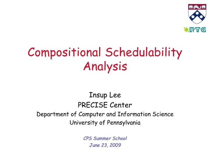
Compositional Schedulability Analysis. Insup Lee PRECISE Center Department of Computer and Information Science University of Pennsylvania CPS Summer School June 23, 2009. Motivation. Hierarchical real-time systems: Need, example, and model. Compositional schedulability analysis

E N D
Compositional Schedulability Analysis Insup Lee PRECISE Center Department of Computer and Information Science University of Pennsylvania CPS Summer School June 23, 2009
Motivation Hierarchical real-time systems: Need, example, and model • Compositional schedulability analysis • Resource model based analysis • Periodic resource models Periodic resource model • Shortcomings of periodic resource • Explicit Deadline Periodic (EDP) resource EDP resource model • Motivation: Need and definitions • Periodic resource based analysis Incremental analysis Characterization of optimality in compositional schedulability analysis Resource optimality Virtual processor cluster-based scheduling on multiprocessors Multiprocessor clustering Summary and research directions Conclusions CSA Tutorial
Motivation • Application domain: embedded systems • complex, networked, and large-scale • Important features of the domain: • module development followed by integration • rapid development cycles, module reuse • resource constraints are critical • Component-based development helps to contain complexity • Goal: resource-sensitive component framework CSA Tutorial
Component technologies • Enable component-based development • abstract components through interfaces • Interfaces preserve intellectual property • compose components preserving compositionality • facilitate modularity, portability, and reusability • Current focus: functional, behavioral aspects • need: non-functional aspects, such as timeliness, reliability, safety, and resource use CSA Tutorial
Motivating example: ARINC 653 P11 ,…,P1m1 P21 ,…,P1m2 Pn1 ,…,Pnmn Process level schedules Partition 1 Partition 2 . . . Partition n Partition level schedule Core module hardware CSA Tutorial
ARINC 653: Schedulability P11 ,…,P1m1 P21 ,…,P1m2 Pn1 ,…,Pnmn Process level schedules Partition 1 Partition 2 . . . Partition n Partition level schedule Core module hardware CSA Tutorial
ARINC 653: Refinement P11 ,…,P1m1 P21 ,…,P1m2 Pn1 ,…,Pnmn P’n1 ,…,P’nmn Process level schedules Partition 1 Partition 2 . . . Partition n Partition level schedule Core module hardware CSA Tutorial
ARINC 653: Incremental analysis P11 ,…,P1m1 P21 ,…,P1m2 Pn1 ,…,Pnmn Process level schedules Partition 1 Partition 2 . . . Partition n Partition level schedule Core module hardware CSA Tutorial
Real-time Components • Workload • Primitive: periodic or sporadic tasks • Composite: other components • Scheduling algorithm • Earliest deadline first (EDF) • Always, job with earliest deadline executes • Deadline monotonic (DM) Assume D ≤ T • Always, job with smallest deadline executes ARINC 653 Partition Component ARINC 653 Process Periodic task CSA Tutorial
(4,1) 0 1 2 3 4 5 6 7 8 9 10 (4,1) 0 1 2 3 4 5 6 7 8 9 10 Real-Time Workload • Set of real-time jobs with hard deadlines • Periodic task specification: T = (p,e) • Sporadic task specification: T = (p,e) • In general: workload depends on contents of the component and scheduling algorithm CSA Tutorial
Hierarchical Scheduling Framework Resource allocation from parent to child Notations Leaf C1,C2,C3 Non-leaf C4,C5 Root C5 ARINC 653 Two-level hierarchical framework Sporadic tasks C1 C4 C3 C5 EDF EDF EDF DM C2 DM Periodic tasks Sporadic tasks CSA Tutorial
Compositional Schedulability Analysis • The problem statement • Analyze the schedulability of component-based real-time systems, where each component has its own scheduler, in a compositional way, i.e., through component interfaces • Component abstraction • Abstract timing and resource requirements of components with interfaces • Interfaces should expose only so much information as is required for analysis • Component composition • Composable interface for real-time embedded systems • Compose component interfaces - to combine timing and resource requirements of components CSA Tutorial
Periodic (10,2) Periodic (15,2) Component interface EDF Two Problems: Abstraction & Composition • Abstraction Problem: abstracts the real-time requirements of component (application) with interface • Compute the minimum real-time requirements necessary for guaranteeing the schedulability of a component CSA Tutorial
Real-Time Task Java Virtual Machine Multimedia T2(33,10) T1(25,5) Real-Time Demand Digital Controller J1(50,3) J2(75,5) CPU OS Scheduler’s Viewpoint VM Scheduler OS Scheduler CSA Tutorial
component interface component interface component interface Two Problems: Abstraction & Composition • Composition Problem: composes component-level properties into system-level (or next-level component) properties scheduling algorithm CSA Tutorial
Compositionality • Compositionality: • system-level properties can be established by composing independently analyzed component-level properties • Compositional reasoning based on assume/guarantee paradigm • components are combined to form a system such that properties established at the component-level still hold at the system level. • Compositional schedulability analysis using the demand/supply bounds • Establish the system-level timing properties by combining component-level timing properties through interfaces CSA Tutorial
Real-time demand composition • Combine real-time requirements of multiple tasks into real-time requirement of a single task Real-Time Constraint Real-Time Constraint Real-Time Constraint Periodic Constraint Periodic Constraint Periodic Constraint EDF / RM CSA Tutorial
Non-composable periodic models? • What are right abstraction levels for real-time compenents? • (execution time, period) • P1 = (p1,e1); e.g., (3,1) • P2 = (p2,e2); e.g., (7,1) • What is P1 || P2? • (LCM(p1,p2), e1*n1 + e2*n2); e.g., (21,10) where n1*p1 = n2*p2 = LCM(p1,p2) • What is the problem? • beh(P1) || beh(P2) = beh(P1||P2)? • Compositionality • (P1 || P2) || P3 = P || P3, where P = P1 || P2 CSA Tutorial
0 1 2 3 4 5 6 7 8 9 Simple Observation (1) • Given a task group G such that • Scheduling algorithm : EDF • A set of periodic tasks : { T1(3,1), T2(7,1) }, model the timing requirements of the task group with a periodic task model • G (3, 1.43) based on utilization does not work !! Deadline miss for T2 CSA Tutorial
0 1 2 3 4 5 6 7 8 9 Simple Observation (2) • Given a task group G such that • Scheduling algorithm : EDF • A set of periodic tasks : { T1(3,1), T2(7,1) }, model the timing requirements of the task group with a periodic task model • G (3, 2.01) works !! CSA Tutorial
Resource Demand Bound • Resource demand bound during an interval of length t • dbf(W,A,t) computes the maximum possibleresource demandthat Wrequires under algorithm A during atime interval of lengtht • Periodic task model T(p,e) [Liu & Layland, ’73] • characterizes the periodic behavior of resource demand with period p and execution time e • Ex: T(3,2) demand t 0 1 2 3 4 5 6 7 8 9 10 CSA Tutorial
Demand Bound - EDF • For a periodic workload set W = {Ti(pi,ei)}, • dbf (W,A,t) for EDF algorithm [Baruah et al.,‘90] demand t 0 1 2 3 4 5 6 7 8 9 10 CSA Tutorial
Component Abstraction (Example) • Given T1(50,7) and T2(70,9), where W={T1,T2} and U(W) = 0.27, a solution space of a periodic resource Γ(Π,Θ) is CSA Tutorial
Component Abstraction (Example) • An approach to pick one solution out of the solution space • Given a range of Π, we can pick Γ(Π,Θ) such that UΓ is minimized. (for example, 28 ≤ Π ≤ 46) Γ(29, 9.86) Γ(29, 11.60) CSA Tutorial
Periodic (50,7) Periodic (70,9) periodic interface Γ(29, 9.86) EDF Abstraction Overhead • For a scheduling component C(W, Γ(Π,Θ), A), its abstraction overhead (OΓ) is UW=0.27 UΓ=0.34 CSA Tutorial
Abstraction Overhead Bound • For a scheduling component C(W, Γ(Π,Θ), A), its abstraction overhead (OΓ) is • A = EDF • A = RM CSA Tutorial
Abstraction Overhead • Simulation Results • with periodic workloads and periodic resource under EDF/RM • the number of tasks n : 2, 4, 8, 16, 32, 64 • the workload utilization U(W) : 0.2~0.7 • the resource period : represented by k CSA Tutorial
Abstraction Overhead • k= 2, U(W) = 0.4 CSA Tutorial
Task (resource demand) representations CSA Tutorial
Three tank system example Adapted from HTL case study [GIKHS07] CSA Tutorial 09/17/07 32
Three tank system example Dissertation Proposal CSA Tutorial 09/17/07 33
ACSR CSA Tutorial
Questions on computing dbf • How efficiently can we compute dbf (demand bound function)? • Periodic processes, RBT, RTC • tasks specified in timed automata with task models • Process algebra, e.g., ACSR • Composition of tasks vs. compositional dbf computation • dbf (P || Q) vs dbf(P) + dbf(Q) CSA Tutorial
workload workload resource Schedulability Analysis • Schedulability analysis determines whether resource demand, which a workload set requires under a scheduling algorithm resource supply, which available resources provide ≤ scheduler CSA Tutorial
Resource Modeling • Dedicated resource : always available at full capacity • Shared resource : not a dedicated resource • Time-sharing : available at some times • Non-time-sharing : available at fractional capacity 0 time 0 time 0 time CSA Tutorial
Resource Modeling • Time-sharing resources • Bounded-delay resource model [Mok et al., ’01] characterizes a time-sharing resource w.r.t. a non-time- sharing resource • Periodic resource model Γ(Π,Θ) [Shin & Lee, RTSS ’03] characterizes periodic resource allocations - EDP model [Easwaran et all, RTSS 07] time 0 1 2 3 4 5 6 7 8 9 CSA Tutorial
Resource Model Supply • sbfR(t) :the minimumpossible resource supplyof model R over all intervalsof length t • For a given periodic resource modelwe can identify resource allocation pattern corresponding to sbfR(t) • Example below for = (5,3) sbf Blackout interval f f f f f f f f f 0 1 2 3 4 5 6 7 8 9 10 11 12 13 14 15 CSA Tutorial
Supply Bound Function (sbf) • sbf(t) : • lsbf(t) : Linear lower bound of sbf(t) Q Bandwidth Blackout interval lsbf ( t ) ( t ( 2 ) ) = - 2P - Q f 4 1 4 2 4 3 P CSA Tutorial
Resource Satisfiability Analysis (Periodic Resource Model under EDF) • Component C is schedulable under EDF usingperiodic resource model =(,)iff, for all t > 0, dbfC(t)≤lsbf(t)≤ sbf(t) [ShLe03] sbf Bandwidth / lsbf Blackout interval 2(-) dbfC CSA Tutorial
Resource Satisfiability Analysis (Periodic Resource Model under DM) • Component C is schedulable under DM usingperiodic resource model =(,)iff, for all i: 1 ≤ i ≤ n, there exists ti s.t., rbfC,i(ti)≤lsbf(ti)≤ sbf(ti) [ShLe03] sbf rbfC,i lsbf CSA Tutorial
What are they? • Explicit Deadline Periodic resource • Model: = (,,) • Explicit deadline • resource units in time units • Repeat supply every time units • Properties • Periodic resource model is a EDP model with = • Maximum slack of EDP model depends on and for a fixed • Slack can be controlled using without changing bandwidth of model (within limits) • Smaller bandwidth required to schedule the same component, when compared to periodicresource models • improves precision of resource allocation AFOSR PI Meeting
Supply bound function (sbf) • sbf(t) • lsbf(t) Q lsbf ( t ) ( t ( 2 ) ) = - P + D - Q W P Bandwidth Starvation length AFOSR PI Meeting
Supply bound function (sbf) Starvation length = 4 G(5,3) time 0 4 5 9 Starvation length = 3 (5,3,4) time 0 4 5 9 AFOSR PI Meeting
Bandwidth optimal interface • Given component C and period • Compute and • Relation between and desired • We usebandwidth optimality • Minimizes resource bandwidth / • Occurs when = (Theorem 3.2 in RTSS’07) AFOSR PI Meeting
Bandwidth optimal interface sbf’ ’ = (,,), > dbfC minimum bandwidth for model ’ AFOSR PI Meeting
= (,,) • can be reduced Bandwidth optimal interface dbfC AFOSR PI Meeting
= (,*,*) sbf bandwidth optimal model Bandwidth optimal interface dbfC AFOSR PI Meeting