Download
1 / 19
300 likes | 584 Views
Chapter 11 Project Analysis and Evaluation. Homework: 19, 25 & 26. Lecture Organization. Scenario and Other “What-If” Analyses Break-Even Analysis Additional Considerations in Capital Budgeting. Evaluating NPV Estimates. The Basic Problem: How reliable is our NPV estimate?

E N D
Chapter 11Project Analysis and Evaluation • Homework: 19, 25 & 26
Lecture Organization • Scenario and Other “What-If” Analyses • Break-Even Analysis • Additional Considerations in Capital Budgeting
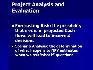
Evaluating NPV Estimates • The Basic Problem: How reliable is our NPV estimate? • Projected vs. actual cash flows Estimated cash flows are based on a distribution of possible outcomes each period • Forecasting risk The possibility of a bad decision due to errors in cash flow projections
Scenario and Other “What-If” Analyses • “Base case” estimation Estimated NPV based on initial cash flow projections • Scenario analysis Posit best- and worst-case scenarios and calculate NPVs • Sensitivity analysis How does the estimated NPV change when one of the input variables changes? • Simulation analysis Vary several input variables simultaneously, then construct a distribution of possible NPV estimates
Fairways Driving Range Example • Fairways Driving Range expects rentals to be 20,000 buckets at $3 per bucket. Equipment costs are $20,000 depreciated using SL over 5 years and have a $0 salvage value. Variable costs are 10% of rentals and fixed costs are $45,000 per year. Assume no increase in working capital nor any additional capital outlays. The required return is 15% and the tax rate is 15%. Revenues $60,000 Variable Costs 6,000 Fixed Costs 45,000 EBIT 5,000 Taxes (@15%) 750 Net Income $ 4,250
Fairways Driving Range Example (concluded) • Estimated annual cash inflows: • At 15%, the base-case NPV is:
Fairways Driving Range Scenario Analysis INPUTS FOR SCENARIO ANALYSIS • Base Case: Rentals are 20,000 buckets, variable costs are 10% of revenues, fixed costs are $45,000, depreciation is $4,000 per year, and the tax rate is 15%. • Best Case: Rentals are 25,000 buckets, variable costs are 8% of revenues, fixed costs are $45,000, depreciation is $4,000 per year, and the tax rate is 15%. • Worst Case: Rentals are 15,000 buckets, variable costs are 12% of revenues, fixed costs are $45,000, depreciation is $4,000 per year, and the tax rate is 15%.
Fairways Driving Range Scenario Analysis (concluded) Scenario Rentals Revenues Net Income Cash Flow Best Case 25,000 $75,000 $17,000 $21,000 Base Case 20,000 60,000 4,250 8,250 Worst Case 15,000 45,000 -9,400 -5,400 Note that the worst case results in a tax credit. This assumes that the owners had other income against which the loss is offset.
Fairways Driving Range Sensitivity Analysis • Base Case: Rentals are 20,000 buckets, variable costs are 10% of revenues, fixed costs are $45,000, depreciation is $4,000 per year, and the tax rate is 15%. • Best Case: Rentals are 25,000 buckets and revenues are $75,000. All other variables are unchanged. • Worst Case: Rentals are 15,000 buckets and revenues are $45,000. All other variables are unchanged.
Fairways Driving Range Sensitivity Analysis (concluded) Scenario Rentals Revenues Net Income Cash Flow Best Case 25,000 $75,000 $15,725 $19,725 Base Case 20,000 60,000 4,250 8,250 Worst Case 15,000 45,000 -7,225 -3,225 Note that the worst case results in a tax credit. This assumes that the owners had other income against which the loss is offset.
Fairways Driving Range: Rentals vs. NPV Fairways Sensitivity Analysis - Rentals vs. NPV NPV Best case NPV = $46,120 $60,000 x Base case NPV = $7,655 x 0 Worst case NPV = -$30,810 x -$60,000 25,000 15,000 20,000 Rentals per Year
Fairways Driving Range: Total Cost Calculations • Total Cost = Variable cost + Fixed cost Rentals Variable Cost Fixed Cost Total Cost 0 $0 $45,000 $45,000 15,000 4,500 45,000 49,500 20,000 6,000 45,000 51,000 25,000 7,500 45,000 52,500
Fairways Driving Range: Break-Even Analysis Fairways Break-Even Analysis - Sales vs. Costs and Rentals Sales and Costs Total Revenues $80,000 Break-Even Point 18,148 Buckets Net Income > 0 $50,000 Net Income < 0 $20,000 25,000 15,000 20,000 Rentals per Year
Break-Even Measures I. The General Expression Q = (FC + OCF)/(P - v) where: FC = total fixed costs P = Price per unit v = variable cost per unit II. The Accounting Break-Even Point At the Accounting BEP, net income = 0. III. The Cash Break-Even Point At the Cash BEP, operating cash flow = 0. IV. The Financial Break-Even Point
Fairways Driving Range: Accounting Break-Even Quantity • Fairways Accounting Break-Even Quantity (Q) Q = (Fixed costs + depreciation)/(Price per unit - variable cost per unit)
Chapter 11 Quick Quiz Assume you have the following information about Vanover Manufacturing: • Price = $5 per unit; variable costs = $3 per unit • Fixed operating costs = $10,000 • Initial cost is $20,000 • 5 year life; straight-line depreciation to 0, no salvage value • Assume no taxes • Required return = 20%
Chapter 11 Quick Quiz (concluded) • Break-Even Computations A. Accounting Break-Even B. Cash Break-Even B. Financial Break-Even
Degree of Operating Leverage (DOL) DOL = (% change in OCF) / (% change in Q) Higher DOL suggests (smaller/greater) risk in OCF
T11.14 Managerial Options and Capital Budgeting • Managerial options and capital budgeting • What is ignored in a static DCF analysis? Management’s ability to modify the project as events occur. • Contingency planning 1. The option to expand 2. The option to abandon 3. The option to wait Generally, the exclusion of managerial options from the analysis causes us to underestimate the “true” NPV of a project. Why?