Download

1 / 35
350 likes | 483 Views
Chapter Eleven. Project Analysis and Evaluation. Chapter Outline. Evaluating NPV Estimates Scenario and Other What-If Analyses Break-Even Analysis Operating Cash Flow, Sales Volume, and Break-Even Operating Leverage Capital Rationing. Evaluating NPV Estimates.

E N D
Chapter Eleven Project Analysis and Evaluation
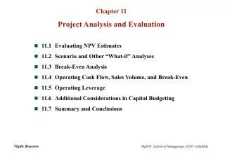
Chapter Outline • Evaluating NPV Estimates • Scenario and Other What-If Analyses • Break-Even Analysis • Operating Cash Flow, Sales Volume, and Break-Even • Operating Leverage • Capital Rationing
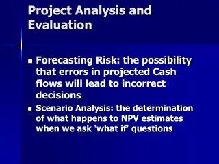
Evaluating NPV Estimates • The NPV estimates are just that – estimates • A positive NPV is a good start – now we need to take a closer look • Forecasting risk (estimation risk)– how sensitive is our NPV to changes in the cash flow estimates, the more sensitive, the greater the forecasting risk • What about the sales forecasts? • Can be manufactured at lower costs? • What about the discount rate? • Positive NPV projects are rare; found one, be suspicious.
What is sensitivity analysis? • Shows how changes in a variable such as unit sales affect NPV or IRR, other things held constant. • Sensitivity analysis begins with a base-case situation – developed using the expected values for each input. • Answers “what if” questions, e.g. “What if sales decline by 30%?”
Sensitivity Analysis -30% $113 $17 $85 -15% $100 $52 $86 0% $88 $88 $88 15% $76 $124 $90 30% $65 $159 $91 Change from Resulting NPV (000s) Base Level r Unit Sales Salvage
NPV (000s) Unit Sales Salvage 88 r -30 -20 -10 Base 10 20 30 Value (%)
Results of Sensitivity Analysis • Steeper sensitivity lines show greater risk. Small changes result in large declines in NPV. • Unit sales line is steeper than salvage value or r, so for this project, should worry most about accuracy of sales forecast.
Advantages - Disadvantages • Disadvantage: • Ignores relationships among variables. • Advantages: • Gives some idea of stand-alone risk. • Identifies dangerous variables. • Gives some breakeven information.
What is scenario analysis? • Examines several possible situations, usually worst case, most likely case, and best case. • Provides a range of possible outcomes.
Best scenario: 1,600 units @ $240Worst scenario: 900 units @ $160 Scenario Probability NPV(000) Probability NPV Best 0.25 $ 279 Base 0.50 88 Worst 0.25 -49 E(NPV) = $101.5 (NPV) = 75.7 CV(NPV) = (NPV)/E(NPV) = 0.75
Are there any problems with scenario analysis? • Only considers a few possible out-comes. • Assumes that inputs are perfectly correlated--all “bad” values occur together and all “good” values occur together.
What is a simulation analysis? • A computerized version of scenario analysis which uses continuous probability distributions. • Computer selects values for each variable based on given probability distributions. (More...)
NPV and IRR are calculated. • Process is repeated many times (1,000 or more). • End result: Probability distribution of NPV and IRR based on sample of simulated values. • Generally shown graphically.
Simulation Example • Assume a: • Normal distribution for unit sales: • Mean = 1,250 • Standard deviation = 200 • Triangular distribution for unit price: • Lower bound = $160 • Most likely = $200 • Upper bound = $250
Simulation Process • Pick a random variable for unit sales and sale price. • Substitute these values in the spreadsheet and calculate NPV. • Repeat the process many times, saving the input variables (units and price) and the output (NPV).
Simulation Results (1000 trials) UnitsPriceNPV Mean 1260 $202 $95,914 St. Dev. 201 $18 $59,875 CV 0.62 Max 1883 $248 $353,238 Min 685 $163 ($45,713) Prob NPV>0 97%
Interpreting the Results • Inputs are consistent with specificied distributions. • Units: Mean = 1260, St. Dev. = 201. • Price: Min = $163, Mean = $202, Max = $248. • Mean NPV = $95,914. • Low probability of negative NPV (100% - 97% = 3%).
What are the advantages of simulation analysis? • Reflects the probability distributions of each input. • Shows range of NPVs, the expected NPV, NPV, and CVNPV. • Gives an intuitive graph of the risk situation.
What are the disadvantages of simulation? • Difficult to specify probability distributions and correlations. • If inputs are bad, output will be bad:“Garbage in, garbage out.” (More...)
Making A Decision • Beware “Paralysis of Analysis” • At some point you have to make a decision • If the majority of your scenarios have positive NPVs, then you can feel reasonably comfortable about accepting the project • If you have a crucial variable that leads to a negative NPV with a small change in the estimates, then you may want to forego the project
Break-Even Analysis and Costs • two types of costs that are important in breakeven analysis: variable and fixed • Total variable costs = quantity * cost per unit • Fixed costs are constant, regardless of output, over some time period • Total costs = fixed + variable = FC + Qv • Example:Your firm pays $3000 per month in fixed costs. You also pay $15 per unit to produce your product. • What is your total cost if you produce 1000 units? • TC = 3000 + 15*1000 = 18,000 • What if you produce 5000 units? • TC = 3000 + 15*5000 = 78,000
Average vs. Marginal Cost • Average Cost • TC / # of units • Will decrease as # of units increases • Marginal Cost • The cost to produce one more unit • Example: What is the average cost and marginal cost under each situation in the previous example • Produce 1000 units: • Average = 18,000 / 1000 = $18, Marginal= 15 • Produce 5000 units: • Average = 78,000 / 5000 = $15.60, Marginal= 15
Break-Even Analysis • There are three common break-even measures: • Accounting break-even – sales volume where net income = 0 • Cash break-even – sales volume where operating cash flow = 0 • Financial break-even – sales volume where net present value = 0
Accounting Break-Even • The quantity that leads to a zero net income: • NI = (Sales – VC – FC – D)(1 – T) = 0 • Now let us ignore taxes. • QP – vQ – FC – D = 0 • Q(P – v) = FC + D • Q = (FC + D) / (P – v) • If a firm just breaks-even on an accounting basis, • cash flow = NI + Depr. = Depr.
Example • Consider the following project • A new product requires an initial investment of $5 million and will be depreciated to an expected salvage of zero over 5 years • The price of the new product is expected to be $25,000 and the variable cost per unit is $15,000 • The fixed cost is $1 million • What is the accounting break-even point each year? • Depreciation = 5,000,000 / 5 = 1,000,000 • Q = (FC + D) / (P – v) • Q = (1,000,000 + 1,000,000)/(25,000 – 15,000) = 200 units • Operatingcash flow = NI + Depr. = 1,000,000
Cash Break-Even • Still no taxes for simplicity. • What is the cash break-even quantity that makes the OCF = 0? • OCF = [(P-v)Q – FC – D] + D = • OCF = (P-v)Q – FC = 0 • QOCF = (FC) / (P – v) • QOCF = (1,000,000) / (25,000 – 15,000) = 100 units
Financial Break-Even Analysis • Consider the previous example • Assume a required return of 18% • What is the financial break-even point (NPV = 0)? • We need to make some assumptions here: Cash flows are the same every year, no salvage and no NWC. If there were salvage and NWC, you would net it out to year 0 so that all you have in future years is OCF. • Similar process to finding the bid price
Financial Break-Even Analysis • What OCF (or payment) makes NPV = 0? • What is the OCF that makes an investment of 5mn$ equal to an annuity for 5 years at 18%? • 5000000 = OCF (PVAF 5, 18%) • OCF = 5000000 / 3.12723 = 1,598,874 • OCF = (P-v)Q – FC • Q = (OCF + FC) / (P – v) • Q = (1,598,874 +1,000,000) / (25,000 – 15,000) = 260 units
Break-Even Analysis Summary • Three common break-even measures: • Accounting break-even = 200 units • (Q = (FC + D) / (P – v); NI = 0; OCF = Depr > 0) • Cash break-even = 100 units • (QOCF = (FC) / (P – v); OCF = 0) • Financial break-even =260 units • (Q = (OCF + FC) / (P – v); NPV = 0) • We are more interested in cash flow than we are in accounting numbers • From the point of project evaluation the question now becomes: Can we sell at least 260 units per year?
Operating Leverage • Operating leverage is the degree to which a project or firm is committed to (relies on) fixed production costs. • The higher the fixed costs, the higher the operating leverage, or vice versa. • Fixed costs act as a lever, ie. A small change in sales can be magnified into a large change in operating cash flows and NPV. • The higher the degree of opearting leverage, the greater is the potential danger from forecasting risk, eg., due to sales forecasts.
Operating leverage is the relationship between sales and operating cash flow • % change in OCF = DOL x % change in Q • DOL = % change in OCF / % change in Q • OCF = Q(P-v) – FC • OCF2 = (Q+1)(P-v) - FC • OCF2 - OCF = (P-v) • DOL = (P-v)/OCF / 1/Q = (P-v) Q/OCF • Or since: OCF + FC = Q(P-v) • DOL = (OCF + FC) / OCF • DOL = 1 + (FC / OCF)
Example: DOL • Consider the previous example • Suppose sales are 260 units • This meets all three break-even measures • What is the DOL at this sales level? • OCF = (25,000 – 15,000)*260 – 1,000,000 = 1,600,000 • DOL = 1 + 1,000,000 / 1,600,000 = 1.625 • What will happen to OCF if unit sales increases by 10%? • Percentage change in OCF = DOL*Percentage change in Q • Percentage change in OCF = 1.625(.1) = .1625 or 16.25% • OCF would increase to 1,600,000(1.1625) = 1,860,000
What will happen to OCF if unit sales decreases by 10%? • Percentage change in OCF = DOL*Percentage change in Q • Percentage change in OCF = 1.625(-.1) = -.1625 or -16.25% • OCF would increase to 1,600,000(0,8375) = 1,340,000 • What is the NPV with OCF= 1,340,000 ? • How can we make it less problematic?