Download
1 / 36
430 likes | 1.21k Views
第一章 系統 TRANSFER FUNCTION 求法的探討. 綱要. 一 . 控制系統的描述 二 . 由電子電路看 TRANSFER FUNCTION 三 . 從控制觀點看 TRANSFER FUNCTION 四 . 由 SIGNAL-FLOW GRAPH 看 TRANSFER FUNCTION 五 . 結論 六 . LFT 求轉移函數之深入探討. 控制系統的描述. 通常一個控制系統的描述方式分為下列三種型態: 1. Transfer function

E N D
綱要 一. 控制系統的描述 二. 由電子電路看TRANSFER FUNCTION 三. 從控制觀點看TRANSFER FUNCTION 四. 由 SIGNAL-FLOW GRAPH 看 TRANSFER FUNCTION 五. 結論 六. LFT求轉移函數之深入探討
控制系統的描述 通常一個控制系統的描述方式分為下列三種型態: 1. Transfer function 2. Zero-pole gain formula 3. State space S-Domain Time - Domain
為何要求轉移函數 求得一系統之轉移函數後,我們才能由其轉移函數對此系統做明確的分析,並進一步得知系統在不同型式命令下之響應 而利用系統輸入及輸出關係求轉移函數之過程,我們稱之為系統建模(system modeling)
一個控制系統的transfer function所代表的是output和input之間的比例:
何謂線性 Transfer function主要的作用為描述控制系統,控制系統之transfer function分析通常只針對 1.線性系統(linear) 2.非時變系統(time-invariant)。 若f(x)為線性(linear)則可表為: f(ax)=af(x) f(x1+x2)=f(x1)+f(x2) 或是f(a1x1+a2x2)=a1f(x1)+a2f(x2) homogenous superposition
由電子電路看轉移函數(觀察法) ZERO-POLE GAIN FORMULA 由下列的電子電路來說明:
(沒有單位) Transfer Function: 電路圖上只要將: Time 趨近無窮( )得到 值 輸出短路(V3=0)得到 輸入短路(V1=0)得到 如此一來就得到系統的transfer function: K
Transfer Function: 利用直接觀察法: 將Time趨近於無窮(s=0) 電容開路 可得 值 EX1.
利用直接觀察法我們可以馬上得知 之值,所以Transfer Function為 可利用 s ∞ double Check 答案
設R1=10Ω;R2=10Ω;R3=10Ω;C=0.01μF; 所畫出的Bode Plot
Transfer Function: 利用直接觀察法: 將Time趨近於無窮(S=0) 電容開路 可得 值 EX2
利用直接觀察法我們可以馬上得知 之值,所以Transfer Function為 可利用 s ∞ double Check 答案
設R1=10Ω;R2=10Ω;R3=10Ω;C=0.01μF; 所畫出的Bode Plot
結論 • 由上述的例題中,我們可以清楚的了解不管是用觀察法或是利用電阻分壓的方式,所得到的Transfer Function的結果均相同,速度上觀察法會比較快,這是因為以上例題屬於簡單的電路,若遇到複雜的電路觀察法可能就不太適用,電阻分壓的方式在任何的電路均適用。 • 觀察法只適用於只有單一儲能元件的電路。
結論 • 觀察法可以讓我們明顯的看出時間常數直接得知波德圖的轉折頻率以及直流增益
從控制觀點看轉移函數(截點法) 原理:應用w=LFT(P,K)r 雙端網路 (two-port network)把原系統轉換成控制系統block diagram的模式 其中 (output) (input) feedback
LFT 雙端網路 解w = LFT(P, K ) r 國立成功大學馬達科技研究中心 蔡明祺教授 NCKU Electric Motor Technology Research Center
LFT 雙端網路 = * ………(1) …………………..(2) 由(1)(2)解聯立 Transfer function,可得:
我們以同一個例題來說明: 將其轉換成控制系統方塊圖:
範例一: 步驟: (1) 系統為了形成一個雙端網路,將系統剪 成open-loop的型式,最理想的模式就是剪 掉 之後,沒有一個迴路可以走的完
(2) 每剪一刀,就多一個輸出、一個輸入,所以要剪幾刀則照步驟1的原則去做 (3) 由系統得到一個矩陣: 求p矩陣之要點: (1)剪斷迴路 (2)起點-終點
(4) 代入公式: (其中 ) 所以跟由OP電路求出的transfer function是相同的!
由Signal-Flow Graph看轉移函數(Manson’s Rule) Signal-flow graph為對於block diagram的簡單標註 基本性質: (1) Signal-flow graph 只應用在線性系統 (2) 信號在branches走的方向以箭號來分辨 (3) Branches的方向由 到 ,而node , 是 dependent (4)
我們再以同一個例題來驗證: 化成signal-flow graph:
signal-flow graph用在transfer function上的關係式為: 其中 M = gain between and = 輸出node的變數 = 輸入node的變數 = forward path的gain △ = 1- (sum of all individual loop gains) + (sum of gain product of all possible combinations of non-touching loops ) △k = The△for that part of the signal-flow graph which is non-touching with the Kth forward path
Three loops are: L1= -1 , L2= -1 , L3= -1/RCs *All loops touch the forward path。 *Loops L1 and L3 are non-touching。 Therefore the transfer function is : 所以求出的transfer function跟前兩種求的皆為相同!
結論 由上述三種不同方法求取同一系統的transfer function,雖然其原理跟求取的過程不盡相同,但是其所求的系統transfer function皆完全相同。所以驗證成功!