Download
1 / 41
420 likes | 535 Views
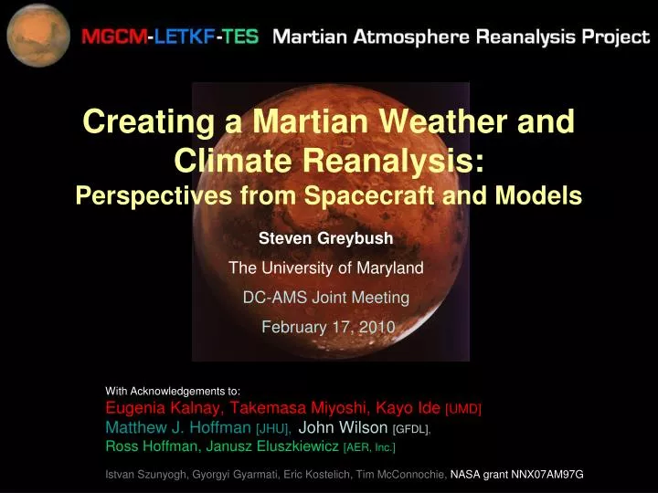
Creating a Martian Weather and Climate Reanalysis: Perspectives from Spacecraft and Models. With Acknowledgements to: Eugenia Kalnay, Takemasa Miyoshi, Kayo Ide [UMD] Matthew J. Hoffman [JHU], John Wilson [GFDL] , Ross Hoffman, Janusz Eluszkiewicz [AER, Inc.]

E N D
Creating a Martian Weather and Climate Reanalysis:Perspectives from Spacecraft and Models With Acknowledgements to: Eugenia Kalnay,Takemasa Miyoshi,Kayo Ide [UMD] Matthew J. Hoffman [JHU], John Wilson [GFDL], Ross Hoffman,Janusz Eluszkiewicz [AER, Inc.] Istvan Szunyogh, Gyorgyi Gyarmati, Eric Kostelich, Tim McConnochie, NASA grant NNX07AM97G Steven Greybush The University of Maryland DC-AMS Joint Meeting February 17, 2010
Outline Basics of Martian Weather and Climate Mars Atmosphere Breeding: Elucidating Atmospheric Instabilities Martian Data Assimilation: Temperatures, and eventually Dust Future Directions for the Mars Reanalysis
Comparing Mars and Earth Table Courtesy of Matthew Hoffman and John Wilson
Martian Topography Vastitas Borealis Olympus Mons Valles Marineris Hellas Basin
Seasons on Mars Elliptic orbit: 44% variation in solar radiation between aphelion & perihelion Slide Courtesy of John Wilson
Exploration of Mars and Relevance for Weather and Climate Mariner Program: Observed Dust Storms Mars Reconnaissance Orbiter: MCS, MARCI… Mars Global Surveyor: TES, MOC, MOLA… Viking Lander: Surface Pressure Time Series 1970 1980 1990 2000 2010 1960 Images Courtesy of Wikipedia
GFDL Mars GCM Uses finite volume dynamical core Latitude-longitude grid 60x36 grid points (6°x5.29° resolution) 28 vertical levels Hybrid p / σ vertical coordinate Tracers for dust and water vapor, with the option for dust radiative feedback
Bred Vector Motivation In chaotic systems, two states that are initially similar grow far apart. There is at least one unstable direction, or pattern, that grows in time. Breeding is a simple method for finding the shapes of these instabilities (errors). The Bred Vector technique was invented by Toth and Kalnay (1993) as a nonlinear, finite time generalization of Lyapunov vectors.
Procedure Bred Vector Procedure Difference from Control Run Step 2: Add an initial perturbation to the nature run. Step 3: Allow the perturbed run to evolve in time using the MCGM. Step 4: Scale the size of the difference between the runs back to the original value. And Repeat… These Differences are the Bred Vectors Day 0 Day 1 … Day 667 Day 668 … Step 1: Create a long nature run (control run) of the MGCM.
MGCM Breeding Experiment Parameters: Rescaling Time Interval: 6 hours Rescaling Amplitude: 1 K Rescaling Norm: Temperature-Squared Norm, Scaled by Cosine Latitude Experiment Length: 1 Martian Year (668 Martian Days) Rescaling only occurs during periods of Bred Vector growth beyond original amplitude. Bred vectors are kept young by adding random perturbation each rescaling interval whose magnitude is 1% of the original perturbation. Fixed dust scenario (opacity = 0.3)
Ls=270 Ls=0 Season labels apply to Northern Hemisphere. Ls=180 Ls=270
Day 078 (Ls= 302, Boreal Winter): BV activity near surface temperature front begins to flare up.
Day 080 (Ls= 304, Boreal Winter): Just two days later, BV now extends vertically along the length of the front. Connection to the upper level tropics begins.
Day 175 (Ls= 358, near boreal vernal equinox): Typical winter BV activity along temperature front with upper level tropical connection. First hint of southern hemisphere activity.
Day 235 (Ls= 22, early boreal spring): Winter BV activity has begun to weaken, as the tropical connection has disappeared.
Day 240 (Ls= 230, early boreal spring): Southern hemisphere activity has now grown rapidly along austral front.
Day 430 (Ls= 116. austral mid-winter): Southern hemisphere BV activity now assumes full spatial extent.
Day 549 (near boreal autumn equinox): Signs BV of activity in the northern hemisphere have resumed.
Day 551 (Ls= 180, boreal autumn equinox): Activity in northern hemisphere has extended vertically.
Day 590 (mid boreal autumn): Activity in both hemispheres, but most intense along southern polar front.
Day 668 (Ls= 252, prior to boreal winter solstice): The seasons have returned full circle, with southern hemisphere activity fading and northern winter dominant.
BV Kinetic Energy Equation • Begin from the equations of motion for the MGCM (momentum equation in sigma coordinates). • Control run and perturbed run both satisfy these equations exactly. • Derive kinetic energy equation for bred vectors (difference between control and perturbed runs). Term 1: Transport of BV KE by the total flow Term 2: Pressure Work Term 3: Baroclinic Conversion Term Term 4: Barotropic Conversion Term Term 5: Coordinate Transform Term
* PRELIMINARY * T1 T2 T3 T4 T5 RHS
Martian Breeding Conclusions Atmospheric instabilities most active in winter and spring hemispheres, particularly along temperature front. System rapidly grows from quiescent to active within a few days. Wavenumber 1 and 2 most dominant, with occasional higher frequency signal. Future Work: Continue interpretation of energy equations to diagnose instability types Breeding with interactive dust scheme
Assimilation of TES Data • Observations from 1999-2005 • Temperature Retrievals at 19 Vertical Levels • Observation Error ~ 3 K • Use of Superobservations Mars Global Surveyor Courtesy NASA/JPL-Caltech Sample locations of TES profiles during 6-hour interval
Thermal Emission Spectrometer Temperature Profiles TES MGCM MGCM MGCM MGCM LETKF Local Ensemble Transform Kalman Filter MGCM MGCM Mars Global Circulation Model … Analysis Ensemble Forecast Ensemble Time
4D LETKF Considers observations at correct hourly timeslot rather than assume that they were taken at 6-hourly intervals. Important for the strong diurnal changes on Mars. Observations: 3D LETKF Forecast: Analysis: Observations: 4D LETKF Forecast: Analysis: Time (hours): 0 1 2 3 4 5 6 7 8 9 10 11 12 13 14 15
LETKF Parameters 30 day assimilation: Day 530 – Day 560 (Northern Hemisphere Autumn) TES Profiles prior to 2001 Dust Storm Temperatures at 19 Vertical Levels 3 K Observation Error Quality Control Threshold (5 * obs error) Superobservations: 1 per grid point Polar Filtering 16 Member Ensemble; Initially from 16 previous model states (at 6-hour intervals) Gaussian Localization: 400 km in horizontal; 0.4 log P in vertical; 3 hours in time 4D-LETKF: 7 time slots (1 per hour) for each 6-hour cycle 10 % Multiplicative Inflation 10 % Additive Inflation (based on differences between randomly selected nearby dates from different years of nature run) Inflation tapers to zero in upper model levels where there is no observation impact Fixed dust distribution, τ=0.3
Free Run (No Assimilation) RMSE (Obs vs. Fcst) Bias (Obs vs. Fcst) Pressure Pressure Latitude Latitude Contours: Ensemble Mean Temperature
LETKF Initial Run RMSE (Obs vs. Fcst) Bias (Obs vs. Fcst) Pressure Pressure Latitude Latitude Contours: Ensemble Mean Temperature
Analysis Ensemble Spread Bred Vector Amplitude Pressure Pressure Latitude Latitude 10% Multiplicative Inflation
Analysis Ensemble Spread 10% Multiplicative Inflation 10% Multiplicative Inflation 10% Additive Inflation 10% Multiplicative Inflation 10% Additive Inflation Dust Varies τ=0.2-0.5 Contours: Ensemble Mean Temperature
Ensembles with different dust (τ=0.2-0.5) RMSE (Obs vs. Fcst) Bias (Obs vs. Fcst) Pressure Pressure Latitude Latitude Contours: Ensemble Mean Temperature
Comparison of Bias Fixed Dust (τ=0.3) Variable Dust (τ=0.2-0.5) Pressure Pressure Latitude Latitude Contours: Ensemble Mean Temperature
Assimilation Conclusions Assimilation system successful at improving temperature errors along polar front and in areas of high instability. Some biases remain in tropical low levels.
Future Work: • Dust Variability and Assimilation • TES Radiance Assimilation • Observation Error Estimation and System Tuning • Comparison to the Oxford Reanalysis Top Image Courtesy of John Wilson Dust Assimilation from TES Dust Opacities and MOC Imagery Dust Lifting Mask Ice Cap Mask