Download
1 / 22
220 likes | 230 Views
EART20170 data analysis lecture 4: estimates and sample sizes. Dr Paul Connolly. Intended learning outcomes. Know how to estimate population parameters from sample statistics : Know how to estimate a population proportion from a sample proportion.

E N D
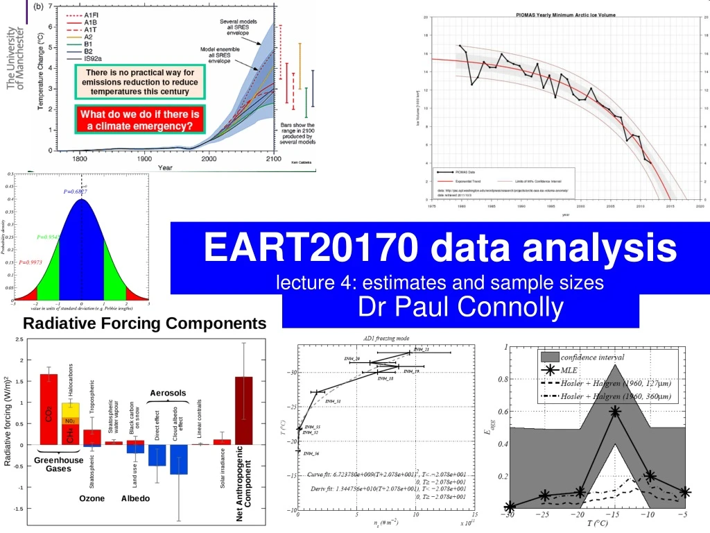
EART20170 data analysislecture 4: estimates and sample sizes Dr Paul Connolly
Intended learning outcomes • Know how to estimate population parameters from sample statistics: • Know how to estimate a population proportion from a sample proportion. • Know how to estimate a population mean from a sample mean.
Definition • `Proportion’ (as in population proportion, sample proportion): the proportion of successes • (eg. the proportion of people who answered yes to: I think Manchester United are the best team – 100%?) • `Margin of error’ amount of error in our measurement (e.g. half the size of the confidence interval). • `Confidence interval’ a range over which we are confident in the value of the statistic.
68.3 % confidence interval 95.5 % confidence interval 99.73 % confidence interval You have come across confidence intervals before (kind of)
Error bars • Scientific papers in the experimental sciences are expected to include error bars on all graphs, though the practice differs somewhat between sciences, and each journal will have its own house style. • Some times researchers will calculate the standard deviation and use that as the error bar, sometime they will calculate the standard error – neither is really appropriate – they should use confidence intervals but it is fine if you say what they are. • How can we do this? => use the normal distribution
Example: climate predictions Different scenarios of temperature change
2013 data! Example: decline of the Arctic sea ice The ice minimum may be zero by 2015!, but at 90% confidence by 2013 or 2018 Ice volume (1000 km3) So what: Well, melting sea ice could switch off the gulf stream and make it colder in the UK Some research says the melting ice may be responsible for the miserable summer and winter snow over the last few years.
Example: attribution of radiative forcing Warming N2O Cooling Intergovernmental Panel on Climate Change For a basic description of the processes (not needed, but interesting?) see: http://130.88.66.117/~mccikpc2/albedo/albedo01.html Username: inuit Password: braunfels
Example: formation of snow See Connolly et al (2012, acp)
Sticking efficiency of snowflakes Why were the results at -15C different to previous results? http://www.youtube.com/watch?v=lAACTET61QY
Example: Nucleation of ice 5 and 95 % confidence intervals Confidence intervals are used throughout scientific investigations. How do we calculate them? Number density of active sites on dust Connolly et al (2009, ACP)
Confidence intervals on proportions Sample proportion of those saying ‘yes’ or vice versa Sample proportion of those saying ‘no’ or vice versa • Statisticians have found that if you have a population of people who either answer yes or no to a question and you take a sample N repeating lots of times the proportion of yes’ that you get is distributed according to a normal distribution (centred on the population proportion) with a standard deviation of: • This means that we can calculate a bound on what the true proportion is within, a `margin of error’: • Thus the confidence interval is: za/2 is the z-value from the normal distribution for a level of significance
Typical problem • You conduct a survey where you ask people a question “Do you believe in human induced climate change?”. • 10 SEAES students are surveyed and 7 say they do believe in human induced climate change. • You want to say something about the population of people you ask (e.g. the majority of students in SEAES do believe in human induced climate change, but you don’t want to ask everyone) • You want to be 95% confident about your statement • How can you do this? • Calculate the confidence interval at some level of confidence: • z(0.05/2)=norminv(0.025,0,1)=-1.96 (ignore sign: 1.96) • p=0.7, q=0.3, N=10 so sqrt(0.7*0.3/10)=0.14 • E=1.96*0.14=0.284 • So 0.416<p<0.984, so we can’t say that p is greater than 0.5 definitively. Try asking more people.
Because: • Designing your experiment: You can use this to estimate what sample size you need to be able to say something definitively.
Note that the 0.25 comes from the fact that the largest value of pxq=0.25, so this is where we require the largest sample size, N (a conservative estimate). • Why is this choice of pxq conservative? Because it results in the largest value of N
Confidence intervals on sample means • is the standard deviation of the population za/2 is the z-value from the normal distribution for a level of significance • Statisticians have found that if you take a sample (size N) from a population of data (e.g. the height of people in UK) and calculate the sample mean, then repeat this lots of times you will get data that are normally distributed about the true mean with a standard deviation of: • This means that the `margin of error’: • And the confidence interval is:
Take random sample size 10, lots of times with m=160 and s=30: Sample 1Sample 2Sample 3Sample 4Sample 5 … 172.1448 147.1493 167.9711 97.6137 119.9242 203.9849 177.3630 144.6987 142.2127 121.5161 140.4469 153.2537 136.3044 170.0316 167.4063 129.3357 188.0844 178.3587 183.1927 147.0068 155.2324 104.1217 156.1121 160.1862 156.7362 157.1232 169.7884 182.8704 181.5937 135.4680 159.8729 102.1456 204.4996 153.5155 165.2333 167.2131 163.2233 162.9584 149.6851 138.0430 144.8713 127.1787 118.4012 129.8534 173.4739 163.2227 210.2701 124.0848 172.7684 172.7456 Means: 159.3448 154.2578 157.6259 154.0653 149.7553 … The most probable value is on the mean, but the standard deviation is s/sqrt(N), therefore can choose confidence level for an error bar
Gold seam at Matilda, Australia (April 2012) http://www.resourcesroadhouse.com.au/_blog/Resources_Roadhouse/post/Blackham_fires_up_new_drilling_program_at_Matilda/
`Environmental’ examplecould apply to grain / clast size in geology or mineral content of sections • Imagine you are assessing the air quality near a gasification plant. They need to conform to air quality directives set by the EC. • Air quality is determined by several different methods. One is excedance of a pollutant over the course of a certain length of time (e.g. over the course of 24 hours). • But often it can be difficult to get continuous measurements. The EC directive for PM10 is 0.05 mg m-3 of air over 24 hours. • 5 measurements are made throughout the day: • 0.06, 0.07, 0.050, 0.055, 0.045 mg m-3. • Is the PM10 over 24 hours clearly over 0.05 mg m-3? • In this example the sample mean is 0.0560, so clearly over 0.05. But have we gathered enough data to say anything really? The standard dev is 0.0096
Set a 95% confidence level, 5% significance level: • NORMINV(0.05/2,0,1)=-1.96 (ignore sign: 1.96) • Why is 0.05 divided by two? • Calculate the margin of error • Note in this example you don’t know the population standard dev so estimate it with the sample standard dev. ~ 0.0096 • Therefore: E=1.96*0.0096/sqrt(5)=0.0084 • So our confidence interval is: 0.0476 < m < 0.0644 (mean=0.0560) • So it isn’t clear that the mean is greater than 0.05 mg m-3
Another important point(for tomorrow’s assessment) • If you are given the upper and lower confidence intervals you can calculate both the best point estimate and the margin of error: • Also note the best point estimate of the population mean is the sample mean. Why? • Because taking lots of sample means produces a distribution centred on the population mean, so there is a good chance a sample mean will be close to the population mean
You will have to open a spreadsheet and calculate some basic stats • You can use either MATLAB or Excel. • Make sure you can remember how to read the sheet and calculate means and standard deviations of a column. • WE ARE IN THE CHEMISTRY CLUSTER TOMORROW 10-12