Download
1 / 125
1.29k likes | 1.53k Views
Chapter 7 Estimates and Sample Sizes. 7-1 Review and Preview 7-2 Estimating a Population Proportion 7-3 Estimating a Population Mean: σ Known (OMIT) 7-4 Estimating a Population Mean: σ Not Known 7-5 Estimating a Population Variance (OMIT). Section 7-1 Review and Preview. Review.

E N D
Chapter 7Estimates and Sample Sizes 7-1 Review and Preview 7-2 Estimating a Population Proportion 7-3 Estimating a Population Mean: σ Known (OMIT) 7-4 Estimating a Population Mean: σ Not Known 7-5 Estimating a Population Variance (OMIT)
Section 7-1 Review and Preview
Review • Chapters 2 & 3 we used “descriptive statistics” when we summarized data using tools such as graphs, and statistics such as the mean and standard deviation. • Chapter 6 we introduced critical values:z denotes the z score with an area of to its right.If = 0.025, the critical value is z0.025 = 1.96.That is, the critical value z0.025 = 1.96 has an area of 0.025 to its right.
Preview This chapter presents the beginning of inferential statistics. • The two major activities of inferential statistics are (1) to use sample data to estimate values of a population parameters, and (2) to test hypotheses or claims made about population parameters. • We introduce methods for estimating values of these important population parameters: proportions, means, and variances. • We also present methods for determining sample sizes necessary to estimate those parameters.
Section 7-2 Estimating a Population Proportion
Key Concept In this section we present methods for using a sample proportion to estimate the value of a population proportion. • The sample proportion is the best point estimate of the population proportion. • We can use a sample proportion to construct a confidence interval to estimate the true value of a population proportion, and we should know how to interpret such confidence intervals. • We should know how to find the sample size necessary to estimate a population proportion.
Definition A point estimate is a single value (or point) used to approximate a population parameter.
The sample proportion p is the best point estimate of the population proportion p. Definition ˆ
Example: Because the sample proportion is the best point estimate of the population proportion, we conclude that the best point estimate of p is 0.70. When using the sample results to estimate the percentage of all adults in the United States who believe in global warming, the best estimate is 70%. In the Chapter Problem (page 314) we noted that in a Pew Research Center poll, 70% of 1501 randomly selected adults in the United States believe in global warming, so the sample proportion is = 0.70. Find the best point estimate of the proportion of all adults in the United States who believe in global warming.
Definition A confidence interval (or interval estimate) is a range (or an interval) of values used to estimate the true value of a population parameter. A confidence interval is sometimes abbreviated as CI. Here is an example of a confidence interval for the population proportion parameter:
NOTE We will learn how to construct confidence intervals from a sample statistic later using a formula.
We must be careful to interpret confidence intervals correctly. There is a correct interpretation and many different and creative incorrect interpretations of the confidence interval a < p < b Typically, we interpret the 95% confidence interval as follows: “We are 95% confident that the interval from a to b actually does contain the true value of the population proportion p.” Interpreting a Confidence Interval
This means that if we were to select many different samples of the same size and construct the corresponding confidence intervals, 95% of them would actually contain the value of the population proportion p. (Note that in this correct interpretation, the level of 95% refers to the success rate of the process being used to estimate the proportion.) Interpreting a Confidence Interval
For example, if we calculate the 95% confidence intervals for 20 different samples of a population, we expect that 95% of the 20 samples, or 19 samples, would have confidence intervals that contain the true value of p. Interpreting a Confidence Interval
Consider the chapter problem example (global warming) again. Suppose we know the true proportion of all adults who believe in global warming is p=0.75 With 95% confidence interval, if we sample 20 times we may compute a confidence interval which does not actually contain p=0.75, such as, but, 19 times out of 20 we would find confidence intervals that do contain p=0.75. This is illustrated in Figure 7-1. Interpreting a Confidence Interval
page 319, Figure 7-1 Interpreting a Confidence Interval
Know the correct interpretation of a confidence interval. Caution
NEXT We will learn now discuss how to construct confidence intervals from a sample statistic.
Critical Values A standard z score can be used to distinguish between sample statistics that are likely to occur and those that are unlikely to occur. Such a z score is called a critical value. Critical values are based on the following observations: Under certain conditions, the sampling distribution of sample proportions can be approximated by a normal distribution.
Critical Values DEFINE: A z score of associated with a sample proportion has a probability of /2 of falling in the right tail. Therefore: • To find , find the z-score in Table A-2 that corresponds to an area of
Example Page 328, problem 7 Find z/2for =0.10
Example Page 328, problem 7 ANSWER:
Definition A critical value is the number on the borderline separating sample statistics that are likely to occur from those that are unlikely to occur. The number z/2 is a critical value that is a z score with the property that it separates an area of /2in the right tail of the standard normal distribution.
Critical Value Because the standard normal distribution is symmetric about the value of z=0, the value of –z/2is at the vertical boundary for thearea of/2in the left tail
The Critical Value z2 -z/2
A confidence level is the probability 1 – (often expressed as the equivalent percentage value) that the confidence interval actually does contain the population parameter, assuming that the estimation process is repeated a large number of times. (The confidence level is also called degree of confidence, or the confidence coefficient.) Definition
Definition Common choices for confidence levels are: 90% confidence level where = 10%, 95% confidence level where = 5%, 99% confidence level where = 1%,
Confidence Level For the standard normal distribution a confidence level of P % corresponds to P percent of the area between the values and For example, if , the confidence level is 1-0.05=0.95=95% which gives the z-score and 95% of the area lies between -1.96 and 1.96 –z/2 z/2 = 5%
z2 for a 95% Confidence Level z2 = 1.96 = 0.05
z2 for a 95% Confidence Level z2 -z2 Critical Values = 5% 2 = 2.5% = .025
Definition When data from a simple random sample are used to estimate a population proportion p, the margin of error, denoted by E, is the maximum likely difference (with probability 1 – , such as 0.95) between the observed proportion and the true value of the population proportion p. The margin of error E is also called the maximum error of the estimate and can be found by multiplying the critical value and the standard deviation of the sample proportions:
Confidence Interval for Estimating a Population Proportion p p = population proportion = sample proportion n = number of sample values E = margin of error z/2 = z score separating an area of /2 in the right tail of the standard normal distribution
Requirements for Using a Confidence Interval for Estimating a Population Proportion p 1. The sample is a simple random sample. 2. The conditions for the binomial distribution are satisfied: there is a fixed number of trials, the trials are independent, there are two categories of outcomes, and the probabilities remain constant for each trial. 3. There are at least 5 successes and 5 failures.
Confidence Interval for Estimating a Population Proportion p ˆ p ˆ p p – E < < + E where
Confidence Interval for Estimating a Population Proportion p ˆ p ˆ p p – E < < + E p + E (p – E, p + E) ˆ ˆ ˆ
Round-Off Rule for Confidence Interval Estimates of p Round the confidence interval limits for p to three significant digits.
Example Page 328 Problem 18:
Example Page 328, problem 18 ANSWER: compute the critical value z/2
Example Page 328, problem 18 ANSWER: compute the sample proportion and
Example Page 328, problem 18 ANSWER: compute the margin of error E
Calculator Use • Here is what the solution manual suggests • Calculate first • To use the formula on a TI calculator: • Calculate , press the multiply key, the parentheses key, then 1- ANS (ANS is the 2nd (-) key on bottom row) , then ENTER. This will give z/2
Example • Press the divide key and input the value of n then ENTER. This will give • Press the square root key, then ANS, then ENTER. This will give • Finally press the multiply key then input the value of then ENTER. This will give E z/2
1. Verify that the required assumptions are satisfied. (The sample is a simple random sample, the conditions for the binomial distribution are satisfied, and the normal distribution can be used to approximate the distribution of sample proportions because np 5, and nq 5 are both satisfied.) 2. Refer to Table A-2 and find the critical value z/2 that corresponds to the desired confidence level. 3. Evaluate the margin of error Procedure for Constructing a Confidence Interval for p
4. Using the value of the calculated margin of error, E and the value of the sample proportion, p, find the values of p – Eand p + E. Substitute those values in the general format for the confidence interval: Procedure for Constructing a Confidence Interval for p - cont ˆ ˆ ˆ ˆ ˆ p – E < p < p + E 5. Round the resulting confidence interval limits to three significant digits.
Example Page 328 Problem 22:
Example Page 328, problem 22 95% confidence interval gives = 5%, compute the critical value z/2
Example Page 328, problem 22 compute the sample proportion and
Example Page 328, problem 22 compute the margin of error E
Example Page 328, problem 22 compute the upper and lower limits of the confidence interval upper limit lower limit