Download
1 / 39
390 likes | 396 Views
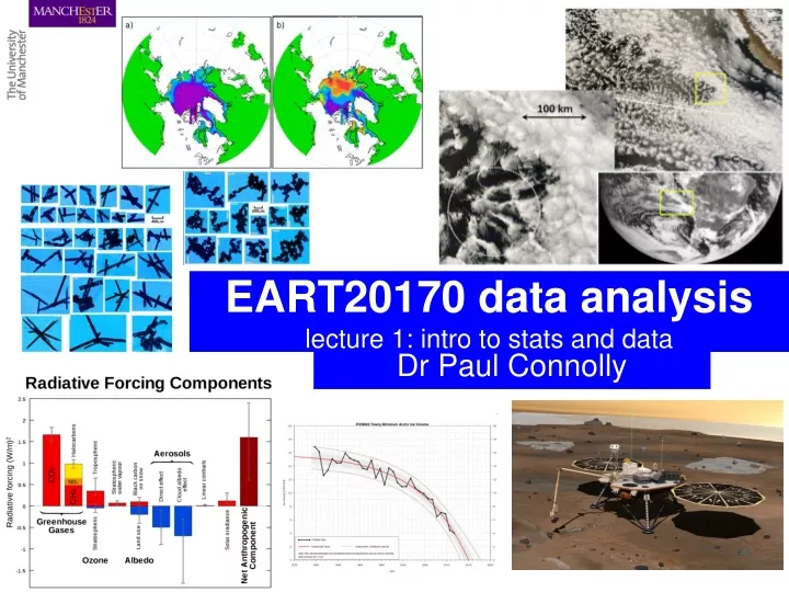
Dr Paul Connolly. EART20170 data analysis lecture 1: intro to stats and data. Outline: Statistics and data. Blackboard and materials Definitions Types of data Common sense approach and attention to detail Investigations and sampling techniques / problems

E N D
Dr Paul Connolly EART20170 data analysislecture 1: intro to stats and data
Outline: Statistics and data • Blackboard and materials • Definitions • Types of data • Common sense approach and attention to detail • Investigations and sampling techniques / problems • Describing and understanding data with histograms and x-y plots • Practical
Definitions • Population • The complete collection of all elements (scores, people, measurements and so on) to be studied; the collection is complete in that it includes all subjects to be studied. • Sample • Sub-collection of members selected from a population. • Census • Collection of data from every member of a population (difficult or impossible)
Dealing with data • The subject of statistics is largely about using sample data to make inferences (or generalisations) about an entire population. • Sample data must be collected in an appropriate way, such as through a process of random selection. • E.g. you could have a biased sample (e.g. traffic survey during rush hour) • Survey of people with an axe to grind • If sample data are not collected in an appropriate way the data may be useless so that not about of statistical torturing can salvage them.
Thinking about your data(common sense really) • Numerical data • Numbers representing counts or measurements. E.g. sizes of cloud drops, grain size, pollution amounts. • Qualitative (or categorical) data • Can be separated into different categories. E.g. genders of academics department http://rchsbowman.wordpress.com/2009/08/12/
Thinking about your data(common sense really) • Numerical data can be: • Discrete data (e.g. number of ice crystals in a cloud). • Continuous data (e.g. the CO2 concentration in the atmosphere). http://rchsbowman.wordpress.com/2009/08/12/
4 Levels of measurement(I’ve yet to use this in any investigations!) • Nominal level of measurement • Data that consist of names, labels or categories (cannot be ranked). • E.g. survey responses (yes or no). • Ordinal level of measurement • Can be ranked, but differences between data can not be determined. • E.g. Course grades, or Moh’s hardness scale. http://www.socialresearchmethods.net/kb/measlevl.php
4 Levels of measurement(I’ve yet to use this in any investigations!) • Interval level of measurement • Like the ordinal scale can be ranked AND differences are meaningful. However, no natural zero starting point. • E.g. years 1000, 2000, 1776 etc. • Temperature on Celsius scale • Ratio level of measurement • Like the interval scale, but with a natural zero • Temperature on Kelvin scale. • Price of text books.
Planning an investigation and working with data(a common sense approach) • Success when planning investigations or working with data often requires more common sense than mathematical expertise. • No point in using a statistical procedure for the sake of it • Good to know about them as sometimes people try to blind you with statistics! • It also requires attention to detail
Common sense # 1 bad samples • Voluntary response sample (or self selected sample) • One in which the respondents themselves decide whether to be included. • E.g. a survey asking whether people believe in human induced global warming. • In this case, valid conclusion can be made only about the specific group of people who agree to take part.
Common sense #2 small samples • Example: associating increased pollution with mortality by measuring one day of PM10 in a city. • Conclusions should not be based on samples that are far too small because you may sample extremes and assume they are typical.
Common sense #4 pictographs • They accentuate the difference by extending both the height and width.
Other misuses of statistics • Correlation is not equal to causality • E.g. CO2 vs temperature. • Most murderers have eaten pickles. Therefore, pickles cause murders. • Virus `link’ to childhood obesity (BBC september 2010). But maybe obese people are more susceptible to virus? • Precise numbers. • E.g. pollution or temperature increased by 65.7142857 % • But the instrumental precision isn’t that good. http://www.norcalblogs.com/watts/2007/01/2006_hottest_year_on_record_so.html
Attention to detail I… Traffic data used as evidence by a traffic consultant in a recent Public Inquiry
Attention to detail II… Air quality modelling used as proof to determine health impacts of an incinerator at a recent Public Inquiry… • The Inspector quashed the development! • However, they are appealing to the high court
Types of investigations(important to get this right!) • Observational study • Observing and measuring specific characteristics without attempting to modify the subjects being studied. • Experiment • Apply some treatment and then observe its effects on the subjects; (subjects in experiments are called experimental units). • E.g. dope cloud drops with volcanic ash in a cloud chamber experiment observe the effects on the cloud
Random (unbiased) sampling(true random sampling is very difficult to do in practice) • Selection so that each individual member has an equal chance of being selected • (e.g. respond to a question in a survey) • or rainfall data over UK (lots of data, every 15 minutes), sample randomly, not biased to times of day, etc – what times would you sample? • Look at boreholes or samples in detail, which ones would you choose? • Choose years to analyse wind data – which years?
Systematic sampling(reasonable compromise, good design) Select some starting point and then select every k th element in the population For example this could be every 5th ice core sample to be taken to the lab for analysis.
Convenience sampling(little statistical validity, poor design) Use results that are easy to get
Stratified sampling(if you wanted to compare groups) • Subdivide the population into at least two different subgroups that share the same characteristics and then draw a sample from each subgroup • E.g. Men vs Women • Cumulus vs stratocumulus (in terms of say precipitation rate) • Are x different or to same as y?
Cluster samplingnever really used myself – seems pretty rubbish to me Divide the population into section (or clusters); randomly select some of those clusters; choose all members from selected clusters.
Errors in investigations • Sampling error (hard to remove) • The difference between a sample result and the true population result; such an error results from chance sample fluctuations (e.g. heights in class) • Non sampling error • Sample data incorrectly collected, recorded or analysed. • E.g. sampled heights of people in class starting at the back of the room (taller people may go to the back of the room?)
Summarising and describing data using histograms and scatter plots
Modelling the flow of traffic Traffic lights Cars – red dots HGVs – green dots Distance along road (m)
Modelling the flow of traffic Traffic lights Do HGVs have an impact on the time it takes for cars to travel down a road? Cars – red dots HGVs – green dots Distance along road (m)
Important! When creating histograms • Create `bins’ to put numerical data into. These should have lower and upper edges • However, the histogram itself is plotted using the bin `mid-points’ • Excel doesn’t do this by default – see YouTube videos on practical and in Blackboard Time it takes for cars to travel down road 156.4547 144.9886 133.8906 129.1142 166.9715 136.7672 126.2964 120.1236 112.3065 108.1506 167.2900 155.0425 …
Positively skewed Negatively skewed Much shorter mode times when there are no HGVs (165 seconds on average) Much longer mode times when there are HGVs (210 seconds on average) Histogram of time-taken to drive down Road 1 HGV every 6 minutes Mode – most common value Mode – most common value Fraction of vehicles
Even causes higher densities at the traffic lights Clusters build up at the site and traffic density / frequency is higher everywhere. Traffic density is higher at the roundabout Histogram of clustering along Road Bi-modal Number of vehicles per 100 m of road per hour tri-modal
What if the HGVs come at a rate of 1 a minute?(a reasonable worse case scenario)
HGVs effectively double the time taken to drive down Road (290s on average) Much shorter times when there are no HGVs (150 seconds on average) Histogram of time-taken to drive down Road (HGV every minute) Negatively skewed Fraction of vehicles
Clusters build up at the site and traffic density / frequency is higher. Traffic density is higher at the roundabout Histogram of clustering along Road (HGV every minute) Number of vehicles per 100 m of road per hour
Cars and HGVs affect the sound level, L(dBA) • Cars are 60 dB(A) at 10 m. • HGVs are 84 dB(A) at 15 m. • Therefore the HGVs will increase the sound level at houses • HGVs can cause clustering of traffic, which can increase or decrease the sound level – this effect is not generally included in noise assessment. • Sound level is important planning criteria
Traffic modelling with steady flow along road(sound data over lap with each other) L10 = 64.0 dB(A) L10 = 61.7 dB(A) L10 = 60.7 dB(A)
Traffic modelling with HGVs slowing(sound levels do not over lap each other) L10 = 72.1 dB(A) L10 = 63.9 dB(A) L10 = 60.7 dB(A)
We will meet you in the Simon building room 6.06 computing practical tomorrow at 10. Please log on to Blackboard and download the practical01.pdf Please bring some head phones if you want to listen to the YouTube videos
Summary • Types of data • Common sense, attention to detail • Investigations / planning, etc. • Histograms, x-y plots • Practicals