Download
1 / 57
580 likes | 714 Views
EART20170 Computing, Data Analysis & Communication skills. Lecturer: Dr Paul Connolly (F18 – Sackville Building) p.connolly@manchester.ac.uk. 1. Data analysis (statistics) 3 lectures & practicals statistics open-book test (2 hours) 2. Computing (Excel statistics/modelling) 2 lectures

E N D
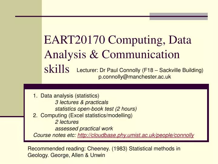
EART20170 Computing, Data Analysis & Communication skills Lecturer: Dr Paul Connolly (F18 – Sackville Building) p.connolly@manchester.ac.uk 1. Data analysis (statistics) 3 lectures & practicals statistics open-book test (2 hours) 2. Computing (Excel statistics/modelling) 2 lectures assessed practical work Course notes etc: http://cloudbase.phy.umist.ac.uk/people/connolly Recommended reading: Cheeney. (1983) Statistical methods in Geology. George, Allen & Unwin
Lecture 1 • Descriptive and inferential statistics • Statistical terms • Scales • Discrete and Continuous data • Accuracy, precision, rounding and errors • Charts • Distributions • Central value, dispersion and symmetry
What are Statistics? • Procedures for organising, summarizing, and interpreting information • Standardized techniques used by scientists • Vocabulary & symbols for communicating about data • A tool box • How do you know which tool to use? (1) What do you want to know? (2) What type of data do you have? • Two main branches: • Descriptive statistics • Inferential statistics
Descriptive and Inferential statistics A. Descriptive Statistics: Tools for summarising, organising, simplifying data Tables & Graphs Measures of Central Tendency Measures of Variability Examples: Average rainfall in Manchester last year Number of car thefts in last year Your test results Percentage of males in our class B. Inferential Statistics: Data from sample used to draw inferences about population Generalising beyond actual observations Generalise from a sample to a population
Statistical terms • Population • complete set of individuals, objects or measurements • Sample • a sub-set of a population • Variable • a characteristic which may take on different values • Data • numbers or measurements collected • A parameter is a characteristic of a population • e.g., the average height of all Britons. • A statistic is a characteristic of a sample • e.g., the average height of a sample of Britons.
Measurement scales • Measurements can be qualitative or quantitative and are measured using four different scales 1. Nominal or categorical scale • uses numbers, names or symbols to classify objects • e.g. classification of soils or rocks
25% difference in hardness 300% difference in hardness 2. Ordinal scale Properties • ranking scale • objects are placed in order • divisions or gaps between objects may no be equal Example: Moh’s hardness scale 1 Talc 2 Gypsum 3 Calcite 4 Fluorite 5 Apatite 6 Orthoclase 7 Quartz 8 Topaz 9 Corundum 10 Diamond
3. Interval scale Properties • equality of length between objects • no true zero Example: Temperature scales Fahrenheit: Fahrenheit established 0°F as the stabilised temperature when equal amounts of ice, water, and salt are mixed. He then defined 96°F as human body temperature. Celsius: 0 and 100 are arbitrarily placed at the melting and boiling points of water. To go between scales is complicated: Interval Scale. You are also allowed to quantify the difference between two interval scale values but there is no natural zero. For example, temperature scales are interval data with 25C warmer than 20C and a 5C difference has some physical meaning. Note that 0C is arbitrary, so that it does not make sense to say that 20C is twice as hot as 10C.
4. Ratio scale Properties • an interval scale with a true zero • ratio of any two scale points are independent of the units of measurement Example: Length (metric/imperial) inches/centimetres = 2.54 miles/kilometres = 1.609344 Ratio Scale. You are also allowed to take ratios among ratio scaled variables. It is now meaningful to say that 10 m is twice as long as 5 m. This ratio hold true regardless of which scale the object is being measured in (e.g. meters or yards). This is because there is a natural zero.
Discrete and Continuous data • Data consisting of numerical (quantitative) variables can be further divided into two groups: discrete and continuous. • If the set of all possible values, when pictured on the number line, consists only of isolated points. • If the set of all values, when pictured on the number line, consists of intervals. • The most common type of discrete variable we will encounter is a counting variable.
Accuracy and precision • Accuracy is the degree of conformity of a measured or calculated quantity to its actual (true) value. • Accuracy is closely related to precision, also called reproducibility or repeatability, the degree to which further measurements or calculations will show the same or similar results. e.g. : using an instrument to measure a property of a rock sample
Accuracy and precision: The target analogy High accuracy but low precision High precision but low accuracy What does High accuracy and high precision look like?
Accuracy and precision:The target analogy High accuracy and high precision
Systematic error Poor accuracy Definite causes Reproducible Random error Poor precision Non-specific causes Not reproducible Two types of error
Systematic error • Diagnosis • Errors have consistent signs • Errors have consistent magnitude • Treatment • Calibration • Correcting procedural flaws • Checking with a different procedure
Random error • Diagnosis • Errors have random sign • Small errors more likely than large errors • Treatment • Take more measurements • Improve technique • Higher instrumental precision
Statistical graphs of data • A picture is worth a thousand words! • Graphs for numerical data: Histograms Frequency polygons Pie • Graphs for categorical data Bar graphs Pie
Histograms • Univariate histograms
Histograms • f on y axis (could also plot p or % ) • X values (or midpoints of class intervals) on x axis • Plot each f with a bar, equal size, touching • No gaps between bars
Frequency Polygons • Frequency Polygons • Depicts information from a frequency table or a grouped frequency table as a line graph
Frequency Polygon A smoothed out histogram Make a point representing f of each value Connect dots Anchor line on x axis Useful for comparing distributions in two samples (in this case, plot p rather than f )
Bar Graphs • For categorical data • Like a histogram, but with gaps between bars • Useful for showing two samples side-by-side
Frequency distribution of random errors • As number of measurements increases the distribution becomes more stable • - The larger the effect the fewer the data you need to identify it • Many measurements of continuous variables show a bell-shaped curve of values this is known as a Gaussian distribution.
Central limit theorem • A quantity produced by the cumulative effect of many independent variables will be approximately Gaussian. • human heights - combined effects of many environmental and genetic factors • weight is non-Gaussian as single factor of how much we eat dominates all others • The Gaussian distribution has some important properties which we will consider in a later lecture. • The central limit theorem can be proved mathematically and empirically.
Central value • Give information concerning the average or typical score of a number of scores • mean • median • mode
Central value: The Mean • The Mean is a measure of central value • What most people mean by “average” • Sum of a set of numbers divided by the number of numbers in the set
Central value: The Mean Arithmetic average: Sample Population
Central value: The Median • Middlemost or most central item in the set of ordered numbers; it separates the distribution into two equal halves • If odd n, middle value of sequence • if X = [1,2,4,6,9,10,12,14,17] • then 9 is the median • If even n, average of 2 middle values • if X = [1,2,4,6,9,10,11,12,14,17] • then 9.5 is the median; i.e., (9+10)/2 • Median is not affected by extreme values
Central value: The Mode • The mode is the most frequently occurring number in a distribution • if X = [1,2,4,7,7,7,8,10,12,14,17] • then 7 is the mode • Easy to see in a simple frequency distribution • Possible to have no modes or more than one mode • bimodal and multimodal • Don’t have to be exactly equal frequency • major mode, minor mode • Mode is not affected by extreme values
When to Use What • Mean is a great measure. But, there are time when its usage is inappropriate or impossible. • Nominal data: Mode • The distribution is bimodal: Mode • You have ordinal data: Median or mode • Are a few extreme scores: Median
Mean Mean Mean Median Mode Mode Mode Median Median Symmetric (Not Skewed) Positively Skewed Negatively Skewed Mean, Median, Mode
Dispersion How tightly clustered or how variable the values are in a data set. Example Data set 1: [0,25,50,75,100] Data set 2: [48,49,50,51,52] Both have a mean of 50, but data set 1 clearly has greater Variability than data set 2. Dispersion
Dispersion: The Range • The Range is one measure of dispersion • The range is the difference between the maximum and minimum values in a set • Example • Data set 1: [1,25,50,75,100]; R: 100-1 +1 = 100 • Data set 2: [48,49,50,51,52]; R: 52-48 + 1= 5 • The range ignores how data are distributed and only takes the extreme scores into account • RANGE = (Xlargest – Xsmallest) + 1
Quartiles • Split Ordered Data into 4 Quarters • = first quartile • = second quartile= Median • = third quartile 25% 25% 25% 25%
Dispersion: Interquartile Range • Difference between third & first quartiles • Interquartile Range = Q3 - Q1 • Spread in middle 50% • Not affected by extreme values
Variance and standard deviation • deviation • squared-deviation • ‘Sum of Squares’ = SS • degrees of freedom Variance: Standard Deviation of sample: Standard Deviation for whole population:
Dispersion: Standard Deviation • let X = [3, 4, 5 ,6, 7] • X = 5 • (X - X) = [-2, -1, 0, 1, 2] • subtract x from each number in X • (X - X)2 = [4, 1, 0, 1, 4] • squared deviations from the mean • S(X - X)2 = 10 • sum of squared deviations from the mean (SS) • S(X - X)2 /n-1 = 10/5 = 2.5 • average squared deviation from the mean • S(X - X)2 /n-1 = 2.5 = 1.58 • square root of averaged squared deviation
Negative skew MODE MEAN=MEDIAN=MODE MEDIAN MEAN Symmetry • Skew - asymmetry Kurtosis - peakedness or flatness
Symmetrical vs. Skewed Frequency Distributions • Symmetrical distribution • Approximately equal numbers of observations above and below the middle • Skewed distribution • One side is more spread out that the other, like a tail • Direction of the skew • Positive or negative (right or left) • Side with the fewer scores • Side that looks like a tail
Symmetric Skewed Right Skewed Left Symmetrical vs. Skewed
Skewed Frequency Distributions • Positively skewed • AKA Skewed right • Tail trails to the right • *** The skew describes the skinny end ***
Skewed Frequency Distributions • Negatively skewed • Skewed left • Tail trails to the left
Symmetry: Skew • The third `moment’ of the distribution • Skewness is a measure of the asymmetry of the probability distribution. Roughly speaking, a distribution has positive skew (right-skewed) if the right (higher value) tail is longer and negative skew (left-skewed) if the left (lower value) tail is longer (confusing the two is a common error).
Symmetry: Kurtosis • The fourth `moment’ of the distribution • A high kurtosis distribution has a sharper "peak" and fatter "tails", while a low kurtosis distribution has a more rounded peak with wider "shoulders".
Accuracy (again!) • Accuracy: the closeness of the measurements to the “actual” or “real” value of the physical quantity. • Statistically this is estimated using the standard error of the mean
The mean of a sample is an estimate of the true (population) mean. » m x The extent to which this estimate differs from the true mean is given by the standard error of the mean s = SE ( x ) N The standard error depends on the standard deviation and the number of measurements 1 N Often it is not possible to reduce the standard deviation significantly (which is limited instrument precision) so repeated measurements (high N) may improve the resolution. Standard error of the mean s = standard deviation of the sample mean and describes the extent to which any single measurement is liable to differ from the mean
Precision (again!) • Precision: is used to indicate the closeness with which the measurements agree with one another. - Statistically the precision is estimated by the standard deviation of the mean • The assessment of the possible error in any measured quantity is of fundamental importance in science. -Precision is related to random errors that can be dealt with using statistics -Accuracy is related to systematic errors and are difficult to deal with using statistics
A set of measurements of the same quantity, each given with a known error ± x s 1 1 The mean value is calculated by “weighting” each of the measurements (x-values) according to its error. ± x s 2 2 ± x s 3 3 ± x s 4 4 ……... with a standard deviation given by 2 å xi si = xtot 2 å 1 si 1 = stot 2 å 1 / si Weighted average