Download
1 / 33
330 likes | 351 Views
Learn about thresholding techniques to convert grayscale images to binary images, and explore component labeling to distinguish objects in binary images.

E N D
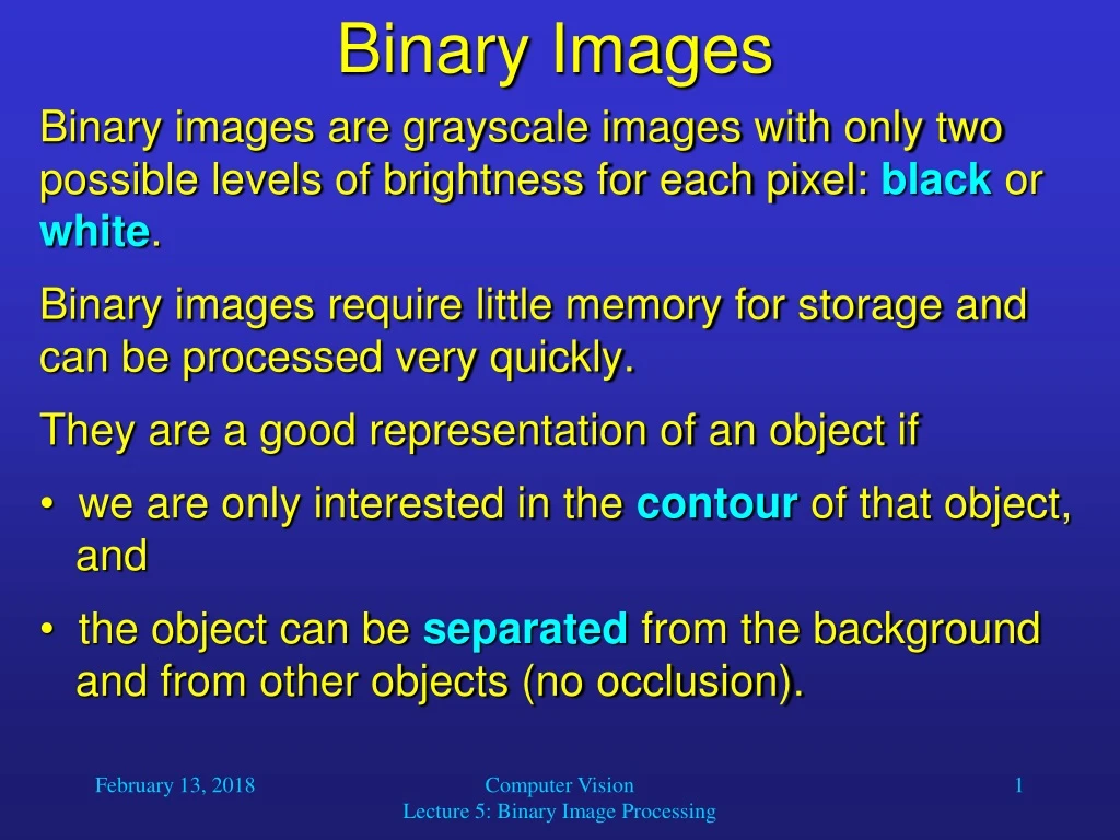
Binary Images • Binary images are grayscale images with only two possible levels of brightness for each pixel: black or white. • Binary images require little memory for storage and can be processed very quickly. • They are a good representation of an object if • we are only interested in the contour of that object, and • the object can be separated from the background and from other objects (no occlusion). Computer Vision Lecture 5: Binary Image Processing
Thresholding • We usually create binary images from grayscale images through thresholding. • This can be done easily and perfectly if, for example, the brightness of pixels is lower for those of the object than for those of the background. • Then we can set a threshold such that is • greater than the brightness value of any object pixel and • smaller than the brightness value of any background pixel. Computer Vision Lecture 5: Binary Image Processing
Thresholding • In that case, we can apply the threshold to the original image A[i, j] to generate the thresholded image A [i, j]: • A[i, j] = 1 if A[i, j] ≤ = 0 otherwise • The convention for binary images is that pixels belonging to the object(s) have value 1 and all other pixels have value 0. • We usually display 1-pixels in black and 0-pixels in white. Computer Vision Lecture 5: Binary Image Processing
Thresholding • If we know that the intensity of all object pixels is in the range between values 1 and 2, we can perform the following thresholding operation: • A [i, j] = 1 if 1≤A[i, j] ≤ 2 = 0 otherwise • If the intensities of all object pixels are not in a particular interval, but are still distinct from the background values, we can do the following: • AZ[i, j] = 1 if A[i, j] Z = 0 otherwise, • Where Z is the set of intensities of object pixels. Computer Vision Lecture 5: Binary Image Processing
Thresholding • Here, the right image is created from the left image by thresholding, assuming that object pixels are darker than background pixels. • As you can see, the result is slightly imperfect (dark background pixels). Computer Vision Lecture 5: Binary Image Processing
Thresholding • How to find the optimal threshold? Computer Vision Lecture 5: Binary Image Processing
Thresholding • Intensity histogram Computer Vision Lecture 5: Binary Image Processing
Thresholding • Thresholding result Computer Vision Lecture 5: Binary Image Processing
Some Definitions [i-1, j] [i-1, j-1] [i-1, j] [i-1, j+1] • For a pixel [i, j] in an image, … [i, j-1] [i, j] [i, j+1] [i, j-1] [i, j] [i, j+1] [i+1, j] [i+1, j-1] [i+1, j] [i+1, j+1] …these are its 4-neighbors (4-neighborhood). …these are its 8-neighbors (8-neighborhood). Computer Vision Lecture 5: Binary Image Processing
8-path 4-path Some Definitions • A path from the pixel at [i0, j0] to the pixel [in, jn] is a sequence of pixel indices [i0, j0], [i1, j1], …, [in, jn] such that the pixel at [ik, jk] is a neighbor of the pixel at [ik+1, jk+1] for all k with 0 ≤k ≤ n – 1. • If the neighbor relation uses 4-connection, then the path is a 4-path; for 8-connection, the path is an 8-path. Computer Vision Lecture 5: Binary Image Processing
Some Definitions • The set of all 1-pixels in an image is called the foreground and is denoted by S. • A pixel pS is said to be connected to qS if there is a path from p to q consisting entirely of pixels of S. • Connectivity is an equivalence relation, because • Pixel p is connected to itself (reflexivity). • If p is connected to q, then q is connected to p (symmetry). • If p is connected to q and q is connected to r, then p is connected to r (transitivity). Computer Vision Lecture 5: Binary Image Processing
Some Definitions • A set of pixels in which each pixel is connected to all other pixels is called a connected component. • The set of all connected components of –S (the complement of S) that have points on the border of an image is called the background. All other components of –S are called holes. 4-connectedness: 4 objects, 1 hole 8-connectedness: 1 object, no hole To avoid ambiguity, use 4-connectedness for foreground and 8-connectedness for background or vice versa. Computer Vision Lecture 5: Binary Image Processing
original image boundary,interior,surround Some Definitions • The boundary of S is the set of pixels of S that have 4-neighbors in –S. The boundary is denoted by S’. • The interior is the set of pixels of S that are not in its boundary. The interior of S is (S – S’). • Region T surrounds region S (or S is inside T), if any 4-path from any point of S to the border of the picture must intersect T. Computer Vision Lecture 5: Binary Image Processing
1 1 2 2 2 1 1 2 2 3 3 3 3 3 3 3 Component Labeling • Component labeling is one of the most fundamental operations on binary images. • It is used to distinguish different objects in an image, for example, bacteria in microscopic images. • We find all connected components in an image and assign a unique label to all pixels in the same component. Computer Vision Lecture 5: Binary Image Processing
Component Labeling • A simple algorithm for labeling connected components works like this: • Scan the image to find an unlabeled 1-pixel and assign it a new label L. • Recursively assign a label L to all its 1-pixel neighbors. • Stop if there are no more unlabeled 1-pixels. • Go to step 1. • However, this algorithm is very inefficient. • Let us develop a more efficient, non-recursive algorithm. Computer Vision Lecture 5: Binary Image Processing
Component Labeling • Scan the image left to right, top to bottom. • If the pixel is 1, then • If only one of its upper and left neighbors has a label, then copy the label. • If both have the same label, then copy the label. • If both have different labels, then copy the upper neighbor’s label and enter both labels in the equivalence table as equivalent labels. • Otherwise assign a new label to this pixel and enter this label in the equivalence table. • If there are more pixels to consider, then go to Step 2. • Find the lowest label for each equivalence set in the equivalence table. • Scan the picture. Replace each label by the lowest label in its equivalence set. Computer Vision Lecture 5: Binary Image Processing
Size Filter • We can use component labeling to remove noise in binary images. • For example, when we want to perform optical character recognition (OCR), it often happens that there are small groups of 1-pixels outside the actual characters. • Since these are usually very small, isolated blobs, we can remove them by applying a size filter, that is, • labeling all components, • computing their size, and • for all components smaller than a threshold , setting all of their pixels to 0. Computer Vision Lecture 5: Binary Image Processing
Size Filter • Here, for = 10, the size filter perfectly removes all noise in the input image. Computer Vision Lecture 5: Binary Image Processing
Size Filter • However, if our threshold is too high, “accidents” may happen. Computer Vision Lecture 5: Binary Image Processing
Size Filter • In the case we had only “positive noise,” that is, there were some 1-pixels in places that should have contained 0-pixels, • Often, we also have “negative noise,” which means that we have 0-pixels in places that should contain 1-pixels. • To remove negative noise, we could define a “hole size filter” that removes all holes that are smaller than a certain threshold. • A common, efficient method of removing both kinds of noise is to apply sequences of expanding and shrinking. Computer Vision Lecture 5: Binary Image Processing
Expanding and Shrinking • As we have just seen, using a size filter is one method for preprocessing images for subsequent character recognition. • Another common way of achieving this is called expanding and shrinking. • Expanding operation: For all pixels in the image, change a pixel from 0 to 1 if any neighbors of the pixel are 1. • Shrinking operation: For all pixels in the image, change a pixel from 1 to 0 if any neighbors of the pixel are 0. Computer Vision Lecture 5: Binary Image Processing
Expanding and Shrinking Here, the original image (left) is expanded (center) or shrunken (right). Shrinking can actually be considered as expanding the background. Computer Vision Lecture 5: Binary Image Processing
Expanding and Shrinking • Expanding followed by shrinking can be used for filling undesirable holes. • Shrinking followed by expanding can be used for removing isolated noise pixels. • If the resolution of the image is sufficiently high and the noise level is low, expanding – shrinking – shrinking – expanding sequence may be able to do both tasks. • Of course we always have to perform the same total number of expanding and shrinking operations. Computer Vision Lecture 5: Binary Image Processing
Expanding and Shrinking Original image Result of expanding followed by shrinking Result of shrinking followed by expanding Computer Vision Lecture 5: Binary Image Processing
Expanding and Shrinking Computer Vision Lecture 5: Binary Image Processing
Compactness • For a two-dimensional continuous geometric figure, its compactness is measured by the quotient P2/A, where p is the figure’s perimeter and A is its area. • For example, for a square of height s we have • P = 4s and A = s2, so its compactness is 16. • For a circle of radius r we have • P = 2r and A = r2, so its compactness is 4 12.56. • No figure is more compact than a circle, so 4 is the minimum value for compactness. • Notice: The more compact a figure is, the lower is its compactness value. Computer Vision Lecture 5: Binary Image Processing
Compactness • For the computation of compactness, the perimeter of a connected component can be defined in different ways: • The sum of lengths of the “cracks” separating pixels of S from pixels of –S. A crack is a line that separates a pair of pixels p and q such that p S and q -S. • The number of steps taken by a boundary- following algorithm. • The number of boundary pixels of S. Computer Vision Lecture 5: Binary Image Processing
Geometric Properties • Let us say that we want to write a program that can recognize different types of tools in binary images. • Then we have the following problem: • The same tool could be shown in different • sizes, • positions, and • orientations. Computer Vision Lecture 5: Binary Image Processing
Geometric Properties Computer Vision Lecture 5: Binary Image Processing
Geometric Properties • We could teach our program what the objects look like at different sizes and orientations, and let the program search all possible positions in the input. • However, that would be a very inefficient and inflexible approach. • Instead, it is much simpler and more efficient to standardize the input before performing object recognition. • We can scale the input object to a given size, center it in the image, and rotate it towards a specific orientation. Computer Vision Lecture 5: Binary Image Processing
Computing Object Size • The size A of an object in a binary image B is simply defined as the number of black pixels (“1-pixels”) in the image: A is also called the zeroth-order moment of the object. In order to standardize the size of the object, we expand or shrink the object so that its size matches a predefined value. Computer Vision Lecture 5: Binary Image Processing
Computing Object Position • We compute the position of an object as the center of gravity of the black pixels: These are also called the first-order moments of the object. In order to standardize the position of the object, we shift its position so that it is in the center of the image. Computer Vision Lecture 5: Binary Image Processing
Computing Object Orientation • We compute the orientation of an object as the orientation of its greatest elongation. • This axis of elongation is also called the axis of second moment of the object. • It is determined as the axis with the least sum of squared distances between the object points and itself. • In order to standardize the orientation of the object, we rotate it around its center so that its axis of second moment is vertical. Computer Vision Lecture 5: Binary Image Processing