Download

1 / 56
560 likes | 765 Views
Regions and Binary Images. Hao Jiang Computer Science Department Sept. 24, 2009. Figure Ground Separation. Brightness Thresholding. Thresholding. Given a grayscale image or an intermediate matrix threshold to create a binary output. Example: background subtraction. -. =.

E N D
Regions and Binary Images Hao Jiang Computer Science Department Sept. 24, 2009
Thresholding • Given a grayscale image or an intermediate matrix threshold to create a binary output. Example: background subtraction - = Looking for pixels that differ significantly from the “empty” background. Slide from Kristen Grauman fg_pix = find(diff > t);
Thresholding • Given a grayscale image or an intermediate matrix threshold to create a binary output. Example: color-based detection fg_pix = find(hue > t1 & hue < t2); Looking for pixels within a certain hue range. Slide from Kristen Grauman
More Binary Images Slide from Kristen Grauman
Issues • How to demarcate multiple regions of interest? • Count objects • Compute further features per object • What to do with “noisy” binary outputs? • Holes • Extra small fragments Slide from Kristen Grauman
Find Connected Regions Our target in this image is the largest blob.
Connected Components • Identify distinct regions of “connected pixels” Shapiro and Stockman
Pixel Neighbors 4 neighboring pixels of the blue pixel
Pixel Neighbors 8 neighboring pixels of the blue pixel
Recursive Method label = 2 for i = 1 to rows for j = 1 to cols if I(i, j) == 1 labelConnectedRegion(i, j, label) label ++; end end
Recursive Method function labelConnectedRegion(int i, int j, int label) if (i,j) is labeled or background or out of boundary return I(i,j)=label for (m,n) belongs to neighbors of (i,j) labelConnectedRegion(m,n,label) end
Two Pass Method • We check each pixel from left to right and up to bottom • If a pixel has no left and up foreground neighbor, we assign a new label to the pixel • If a pixel has only one left or up foreground neighbor, we assign the label of the neighbor to the pixel • If a pixel has both left and up foreground neighbors, and their labels are the same, we assign the label of the neighbor to the pixel • If a pixel has both left and up foreground neighbors, and their labels are the different, we assign the label of the left neighbor to the pixel and use the up-left label pair to update the equivalency table. • We go through another pass to replace the labels to corresponding labels in the equivalency table
Example Image Label equivalence table
Example Image Label equivalence table
Example Image Label equivalence table
Example Image Label equivalence table
Example Image Label equivalence table
Example Image Label equivalence table
Example Image Label equivalence table
Example Image Label equivalence table
Example Image Label equivalence table
Example (2,3) Image Label equivalence table
Example Image Label equivalence table
Example Image Label equivalence table
Example Image Label equivalence table
Example Image Label equivalence table
Example Image Label equivalence table
Example (5,2) Image Label equivalence table
Example Image Label equivalence table
Example Image Label equivalence table
Example Image Label equivalence table
Example Image Label equivalence table
Example Image Label equivalence table
Example Image Label equivalence table
Example (5,2) Image Label equivalence table
Example Image Label equivalence table
Example Image Label equivalence table
Morphology Operations • Define At = { p + t | p is a point in A} • Erosion T = { t | At belongs to S} A Erosion(S, A) S
Morphology Operations • Define At = { p + t | p is a point in A} • Erosion T = { t | At belongs to S} What if A is S
Morphology Operations • Define At = { p + t | p is a point in A} • Dilation T = Union of At and S for all t in S What if A is Erosion(S, A) S
Morphology Operations • Define At = { p + t | p is a point in A} • Dilation T = Union of At and S for all t in S What if A is S
Morphology Operations • Define At = { p + t | p is a point in A} • Dilation T = Union of At and S for all t in S What if A is
Opening • Erode, then dilate • Remove small objects, keep original shape Before opening After opening Slide from Kristen Grauman
Closing • Dilate, then erode • Fill holes, but keep original shape Before closing After closing Slide from Kristen Grauman
Morphology Operators on Grayscale Images • Dilation and erosion typically performed on binary images. • If image is grayscale: for dilation take the neighborhood max, for erosion take the min. eroded original dilated Slide from Kristen Grauman
Matlab • Create structure element se = strel(‘disk’, radius); • Erosion imerode(image, se); • Dilation imdilate(image, se); • Opening imopen(image, se); • Closing imclose(image, se); • More possibilities bwmorph(image, ‘skel’);