Download
1 / 37
370 likes | 376 Views
Binary Images. Each pixel is 0 or 1, background or foreground Image processing to Enhance separation of objects of interest Separate and count multiple objects Understand the shapes of multiple objects. From image to binary image.

E N D
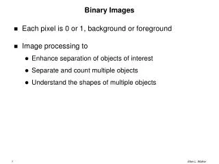
Binary Images • Each pixel is 0 or 1, background or foreground • Image processing to • Enhance separation of objects of interest • Separate and count multiple objects • Understand the shapes of multiple objects
From image to binary image • Classification: dividing pixels into "foreground" and "background" • Thresholding • If a pixel has a value in range (min, max) it is foreground • Often min is 0 or max is maximum pixel value • Choice of range can be manual or automatic • (E.g. look for peaks / valleys in histogram) • More complex operations • Use information from neighboring pixels • Use properties besides pixel value (e.g. location) • …
N W E S Image Neighborhoods • Neighborhoods can be defined for each pixel • The two most common neighborhoods • 4-neighborhood • 8-neighborhood
Applying a Mask • Mask is a set of relative pixel positions. One is designated the origin (0,0) - usually at center • Each mask element is weighted • To apply the mask, put the origin pixel over the image pixel and multiply weights by the pixels under them, then add up all the values. • Usually this is repeated for every image in the pixel. Assumptions must be made for pixels near the edge of the image.
Mask application example • Result is 0 0 0 1 1 0 0 1 2 2 0 1 2 3 2 1 2 3 3 2 2 3 3 3 2 • Mask = 1 1 1, origin at center • Apply to every pixel in image: 0 0 0 0 1 0 0 0 1 1 0 0 1 1 1 0 1 1 1 1 1 1 1 1 1
Masks for object counting • External corners (origin = top left) 0 0 0 0 1 0 0 1 0 1 1 0 0 0 0 0 • Internal corners (origin = top left) 1 1 1 1 1 0 0 1 1 0 0 1 1 1 1 1 • Apply using exact match (result is 1 if every pixel in mask matches the image) • If any of the 4 external corner masks matches, the corner is external (& same for internal)
Counting 4-Connected Objects • The number of 4-connected objects in an image is (E - I) / 4 where E is the number of external corners and I is the number of internal corners. • Assumptions: • Objects are 4-connected (2 diagonal pixels are 2 objects) • Objects do not contain "holes" within them
Connected Components • "Blobs" are connected components • 4-connected (diagonal neighbors don't count) • 8-connected (diagonal neighbors are connected) • The following diagram has 3 4-connected components (red, blue, black) or 2 8-connected components (non-black, black)
Recursive Connected Components • Copy the image • While at least one 1-pixel exists in the existing image • Create a new label • REC_LABEL(label, pixel) • REC_LABEL(label, pixel) • Label and remove the pixel • For each non-zero neighbor • REC_LABEL(label, neighbor)
Recursive Connected Components Example First pixel After 4 recursive calls, no 4-neighbors neighbors to color Start again with a new color on an unmarked pixel
Two-Pass Connected Components • Pass 1 • For every pixel in the image (left-right, top-bottom) • If the pixel is non-zero • If the pixel has no labeled neighbors (above/left) • Create a new label & label it • Else if all labeled neighbors are the same • Give the pixel the same label • Else if neighbors have 2 different labels • Give the pixel the largest label • Mark the smaller label as a parent of the larger one (parent [larger] = smaller)
Two-Pass Connected Components • Pass 2 • Renumber all pixels using only one value for each "equivalence class" • This value is the root of the tree While (parent[x] != 0) x = parent[x];
Two-pass Connected Component Example 2 lines scanned 3 lines scanned 4th line -- Conflict - set black = blue ?
Binary Image Morphology • Morphology = "Study of Shape" • Set of operations that are useful for processing connected components ("blobs") based on shape • Examples • Remove small holes or outcroppings • Remove objects below a given size • Smooth corners
Structuring Element • Mask used for binary morphology • Like convolution masks, they slide over the image and operate on the pixels under them • Common elements: • Box (square or rectangle) • Disk (digital filled circle) • Bar (horizontal or vertical)
Morphology Operations • Dilation • Result is mask OR original • Erosion • Result pixel is 1 if origin pixel is 1 and all pixels covered by the mask are also 1
Morphology Operations • Closing = dilation followed by erosion • Opening = erosion followed by dilation
Applications of Morphology • General • Closing closes holes (up to size of element) • Opening opens spaces (up to size of element) • Specialized • Choose elements of size/shape based on your object • Eliminate objects that are too small / large • Isolate interesting features
Grassfire Transform • Each pixel is distance to closest “1” in the original image.
Two-Pass Algorithm for Grassfire • Set all boundary pixels to Max • First pass: top left to bottom right • If original pixel was 1, pixel is 0 • Else pixel = min(above + 1, left + 1); • Second pass: bottom right to top left • Pixel = min(pixel, below+1,right+1);
Distance Transforms and Medial Axis • Grassfire as described here measures 4-connected distance to the region of interest • Variations • Use a different distance transform, e.g. Euclidean • Use 0 instead of a large value at the boundaries • Medial axis is set of points furthest from a boundary • Set of pixels with maximal values in grassfire • Very sensitive to changes in boundary
Examples • Figure 3.9 (f = dilated, g=grassfire, h=components)
Other Useful Binary Image Operations • Pixelwise AND, OR • Pixelwise Subtraction • 0 if first image is 0, or both images are 1 • Translation • Every pixel is copied (dx, dy) away from its original position
Shape Representation • Shape = list of features • Boundary points, segments • Region features (center, convex hull, etc.) • “Interesting” points, e.g. corners • Shape invariants • Shape = mathematical description • Function type & parameters (e.g. circle, radius 5, centered at (0,0)) • Mathematical function approximation of boundary, e.g. B-spline • Shape Classes
Shape Features • Region features • Simple properties (area, Euler’s #, projections, bounding box, eccentricity, elongatedness, direction, compactness) • Statistical moments • Convex Hull • Region decompositions (hierarchical representation) • Skeleton • Boundary features • Boundary points (e.g. chain code) • Geometric properties (perimeter, curvature, chords, etc.)
Simple Properties • Area • Number of pixels in the region • Perimeter • Number of boundary pixels • Compactness = (Perimeter & Perimeter) / Area • Maximal for circle, minimal for thin, long rectangle • Centroid • Average x value, average y value
Statistical Moments • In a binary image, a moment is the sum of relevant x’s and y’s. • (0,0) moment = area • (1,0) moment / area = average x coordinate • (0,1) moment / area = average y coordinate
Variations on Statistical Moments • Central moment • First translate the shape so that its center is (0,0), i.e. subtract the (average x, average y) values from all pixel locations • Scaled central moment • Divide the central moment by a power of the scale factor and the area • Unscaled central moment • Divide the central moment by a power of the area only
2nd Order Moments and Ellipses • Central (2,0) moment relates to the horizontal axis of an ellipse approximating the shape • Central (0, 2) moment relates to the vertical axis of an ellipse approximating the shape • Central (1,1) moment relates to the rotation of an ellipse approximating the shape
More Region Properties • Bounding box • Min, max x-value, min-max y-value • Extremal points (on the bounding box) • Topmost left, topmost right, leftmost top, leftmost bottom, etc. • Lengths of extremal axes (e.g. top left -> bottom right) • These approximate the Convex Hull of the object • Convex hull is the shape you get by pounding nails into the black pixels and then wrapping them with a rubber band.
Boundary Pixels and Perimeter • 4-connected object (black) • Boundary pixels have at least one white 8-neighbor • 8-connected object (black) • Boundary pixels have at least one white 4-neighbor • If the object is 4-connected, the background is 8-connected and vice versa • Perimeter is the number of boundary pixels • Chain code: start at uppermost, leftmost boundary pixel - list DIRECTION to next pixel until the first one is reached again
Where is the center? • Centroid, center of mass (average x over all pixels, average y over all pixels) • Center of contour (average x, y over boundary pixels only) Example (note sensitivity to contour!)
Region Skeletons • Basis: thinning (many algorithms!) • Maximum values of grassfire transform (medial axis) • Last pixels to disappear with repeated erosion
Hierarchical or Graph Shape Description • Define a set of primitive shapes • Define a set of operations (concatenation, union, intersection, etc.) • Define a shape as a network of primitive shapes (parts) connected by operations • Recognize a shape by recognizing its parts and the relationships between them.
Region Adjacency Graph • Primitive shape = "connected set of pixels" • Operations = "adjacent to" • Element of region 1 is in the neighborhood of element of region 2 • In binary images, all regions with no holes are adjacent to the single background region • All holes are adjacent to the objects that contain them