Download
1 / 54
540 likes | 713 Views
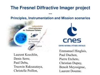
The Fresnel Diffractive Imager project --- Principles, Instrumentation and Mission scenarios. Université de Toulouse, CNRS France. Emmanuel Hinglais, Paul Duchon, Pierre Etcheto, Christian Dupuy, Benoît Meyssignac, Laurent Doumic. Laurent Koechlin, Denis Serre,

E N D
The Fresnel Diffractive Imager project --- Principles, Instrumentation and Mission scenarios Université de Toulouse, CNRS France Emmanuel Hinglais, Paul Duchon, Pierre Etcheto, Christian Dupuy, Benoît Meyssignac, Laurent Doumic. Laurent Koechlin, Denis Serre, Paul Deba, Truswin Raksasataya, Christelle Peillon,
I. Optical Principles Focalization by diffraction Chromatic correction II. Lab prototype, optical and numerical tests High dynamic range Optical setup Tests results on artificial sources Tests planned on sky sources Numerical simulations for large arrays III. Space mission scenarios Orbits and Formation flying configuration Primary array vessel design Focal instrumentation design IV. Astrophysical targets Some of the possible scenarios The Fresnel Diffractive Imager project
Lens (or miror): focusing by refraction (or reflexion) focus Plane wavefront Fresnel array: focusing by diffraction … focus Focalization : different ways Lens Order 0 : plane wave Order 1 : convergent
2D radial expansion Concentric geometry (Soret 1875) Efficiency at order 1: 10% Exemple for 15 Fresnel zones
2D Cartesian expansion Orthogonal geometry (2005) Efficiency at order 1: 4 to 8 % Exemple for 30 Fresnel zones g(x)= 1 si (x2 +f2)1/2Î [(f/ml + (k-off)+1/2) ml ; (f/ml + (k-off)+1) ml[ sinon g(x) = 0 Fresnel Zone plate or Aperture synthesis array ? (here: 1740 ouvertures) Transmission (x, y) = g(x) xor g(y)
Image formation circular geometry => isotropic PSF Image Aperture non linear luminosity scale In order to show the faint isotropic rings.
Image formation Orthogonal geometry => orthogonal PSF Image Aperture Quasi no stray light except in the spikes. Transmission: g(x) g(y) non linear luminosity scale In order to show the faint spikes.
Image formation Case of a second source in the field:
Image formation Case of a second source in the field:
Image formation Case of a second source in the field:
Comparison: Fresnel arrays versus a solid aperture Images of a point source by: 150 Fresnel zones 1500 Fresnel zones Solid square aperture luminosity scale:Power 1/4 to show spikes
"for" Fresnel Arrays: No mirror, no lens to focalize : just vacuum and opaque material. => apotentially very broad operational domain: 90nm - 25 mm Angular resolution: as high as with a mirror the size of the whole array. High dynamic range: 108 on compact objects for a 300 zones array Large tolerance in positioning of subapertures for l/20 wavefront quality: 100 mm in the plane of the array 10 cm in the wave propagation direction (perp. to array) The tolerance is wavelength independent => Opens a way to build very large aberration-free apertures for astrophysics.
"against" Fresnel Arrays: C F = C2/8N l Chromaticity... corrected by small diffractive lens after focus, (order 1 chromaticity cancelled by order -1 chromaticity), but bandpass limitations remain: Dl/l = √2 S/C kilometric focal lengths => requires formation flying in space Low transmission compared to a mirror : t = 5 to 10%
Diffractive lens at order -1 e.g. 10 cm Converging lens e.g. 10 cm 10 to 100 km mask Img. plane 2 : achromatic pupil plane Spacecraft 2 holding focal instrumentation Optical scheme of the Fresnel Diffractive Imager Primary Fresnel array e.g. 20 m Field Optics e.g. 2m Order 0 rays Focal Instrumentation image plane 1dispersed Order 1 rays, focused by primary array Spacecraft 1 holding primary Fresnel array
Chromatically aberrated beam at prime focus The field - bandpas compromise Field delimited by field mirror The chromatic corrector does a good job, but it corrects only what it collects.
II. Lab prototype, optical and numerical test results Prototype built at Observatoire Midi Pyrénées in Toulouse 2006 - 2008
Lab Prototype: light source module • Étoiles doubles • photo • Galaxies en spirales • photo • Gravure : Micro Usinage Laser. source test Exemples de sources test Disque Ø 0,8" d'arc Binaire Disque Ø 32 " d'arc mire 72 " d'arc
Lab prototype: Fresnel array module C = 8 cm 116 zones (26 680 apertures) Opaque foil: inox 80 µm thick Tested in the visible (450-850 nm) F= 23 m for l= 600 nm
Lab prototype, Focal module Field "lens" Order 0 Mask Chromatic correction + doublet focalization Final image 23 m
Lab prototype, focal module, zoom on the corrector lens • 116 zones, 16 mm diameter, Blazed for 600 nm • Fused silica • Résolution selon le plan de la lentille de 1nm, hauteur des marches PTV 1.37 µm • Ion beam etched (SILIOS), 128 levels, • 1 mm "location" precision, 10 nm "depth" precision Diverging Fresnel lens mounted in the optical train
Qualitative results: images of artificial sources broad spectral illumination: 550 - 750 nm uniform Disk 0.8 arc sec uniform Disk 0.8 arc sec with turbulence double source high dynamic range uniform Disk 32 arc sec Galaxy-shaped target 72 arc sec
Quantitative results: measured angular resolution Diffraction limited theoretical profile Sampled optical point spread function The prototype is quasi diffraction limited
Quantitative results: dynamic rangeopticallymeasured versus numerically simulated In these saturated images of a point source, the average background is at 2 *10 -6 Luminosity scaleamplified x1000 Luminosity scaleamplified x1000 8 cm 116 zones Optical image 8 cm 116 zones Numerical Fresnel wave propagation Through all the optical elements The numerical Fresnel propagation tool has been developed for testing large arrays
Quantitative results:PSF of a 300 zones Fresnel Imager (720 000 apertures) numerically simulated Log dynamc range Not apodized, no order 0 mask
Quantitative results:PSF of a 300 zones Fresnel Imager (720 000 apertures) Apodized, order 0 masked numerically simulated Log dynamc range
Quantitative results:PSF of a 300 zones Fresnel Imager (720 000 apertures) Prolate apodized, order 0 masked Log dynamc range 1/4 of the field represented Position in the field (resels)
directionnal " Spergle" type Beyond Orthogonality : improving transmission efficiency and dynamic range
Quantitative results:PSFs of non-orthogonal, square aperture imagers 300 zones, Square aperture cosine apodized, order 0 masked luminosity scale:Power 1/4 to show background
Quantitative results:Convolution simulations 300 zones, Square aperture cosine apodized, order 0 masked The spikes do not degrade extended images PSF HH_30BW, raw image (from HST) HH_30BW, convoluted
III. Space missions scenarios To be proposed for the 2020-2025 period
Generation II prototype: tests on high dynamic rangesky sources Not quite yet XIXth century, 19 meter long, 76 cm Nice Obs refractor
Generation II prototype: tests on the sky 350 zones, 20 cm aperture 20 meter focal, 700 mas resolution 106 or more dynamic range To be built and operated 2008-2010, financed by CNES, subject of a present Ph.D. thesis
"lens" and "receptor" vessels for a 10m circular array configuration Space Missions scenarios:Formation flying configuration
Oor Olp ZOR ZG(étoile) R F L Grand Axe « optique » Zopt xL LP Satellite Récepteur Satellite Lentille de Fresnel ZLP Schéma de principe de l’instrument distribué Space Missions scenarios:Navigation Control Scheme Principe des mesures (2x2 d.d.l. + F) : 1) Le « dépointage » du grand axe optique (Zopt) par rapport à la cible ZGest représenté parDqL. Il permet d’estimer le déport latéral DxL =F. DqL. Sa figuration sur le plan focaldu SSSL (ci-contre) est représenté par l’écart entre le motif des diodes laser implanté sur la grande lentille et la cible stellaire, caractérisée, en fait, par un « motif stellaire » avec ou sans la cible (cachée par la lentille en « contrôle fin »). 2) Le dépointage de l’axe optique du Récepteur par rapport au grand axe optique (DqR) est représenté par l’écart angulaire [ ZOR, ZOPT ]. Plan focal du SSSL dans l’Optique Réceptrice ZG (la cible) Axe Optique du Récepteur : ZOR DqL(= DxL/F) DqR ZOPT(grand axe optique) Lentille de Fresnel Diode Laser 3) Mesure de la distance Focale: En fin de phase d’acquisition, on estimera F à partir de la taille du motif de diodes laser. Par contre, la mesure fine de la focale sera effectuée par télémétrie Laser en phase de contrôle fin.
small Lissajou typically: period: 6 months1 avoidable eclipse every 6 years line of sight ecliptic plane Fresnel lens light shield sun sun 200 000 km Earth ecliptic plane L2 8° acceptable depointing angle of the line of sight = total shield angle protection – Earth, Sun and Moon covering (fonction of the L2 orbit) 14° Moon worst caseevery 28 days Space Missions scenarios:key parameters for spacecraft architecture Orbit and mission • - technology - fabrication- Lissajou orbits - environment - Communications to ground - Vessel to vessel communications fixed RA Antenna & GS Possible a partir de 100 000km from Earth • TM/TC 2 par satellite terre/anti-terre • Liaison RF sensing (type SimbolX) inter-satellite pour la formation • TMI Reflector Array (0 à 40°) • 1 on receptor spacecraft facing earth
Space Missions scenarios: focal instrumentation Intégration of science and navigation channels: privileged Scenarios
Space Missions scenarios: focal instrumentation chromatic correction optics By réfraction By reflection LFC MFCF • NUV+VIS+NIR : lentille de Fresnel blazée à l’ordre –1 qui fonctionne en transmission, suivie d’un doublet convergent et achromatique technologie validée TRL04 : R&T CNES 2004-2007 • UV : miroir de Fresnel blazée à l’ordre –1 ayant double fonction : 1- Réseau correcteur en réflexion et hors axe. 2- Focalisation du faisceau par une concavité globale additionnelle • R&T CNES à venir.
Extra Galactic and Young Universe Scientific Requirements Color Code => Spectral Band : IR NIR Vis NUV FUV
Extra Galactic and Young Universe Instrumentation specifications t =3 h : for Changing Object t = 6 h :for Changing Spectral Band
Active Regions in Our Galaxy Scientific Requirements Distance Between Objects : 0,2° - 0,5° No of Objects per spectral Band : 20 Color Code => Spectral Band : IR NIR Vis NUV FUV
Active Regions in Our Galaxy Instruments specifications IR NIR Vis NUV FUV
Imagery Stellar and Circumstellar With a 500 m array ?
Imagery Stellar and Circumstellar Scientific Requirements IR NIR Vis NUV FUV
Imagery stellar et circumstellar Instrument Specifications IR NIR Vis NUV FUV
Exoplanets Earth @ 10 pc detection and spectroscopy 40m array, 300 Fresnel zones, PIAA, spectral resolution 50, 2*48h exposure time
"Exoplanets" Scientific Requirements IR NIR Vis NUV FUV