Binomial and Poisson Probability Distributions

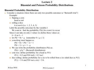
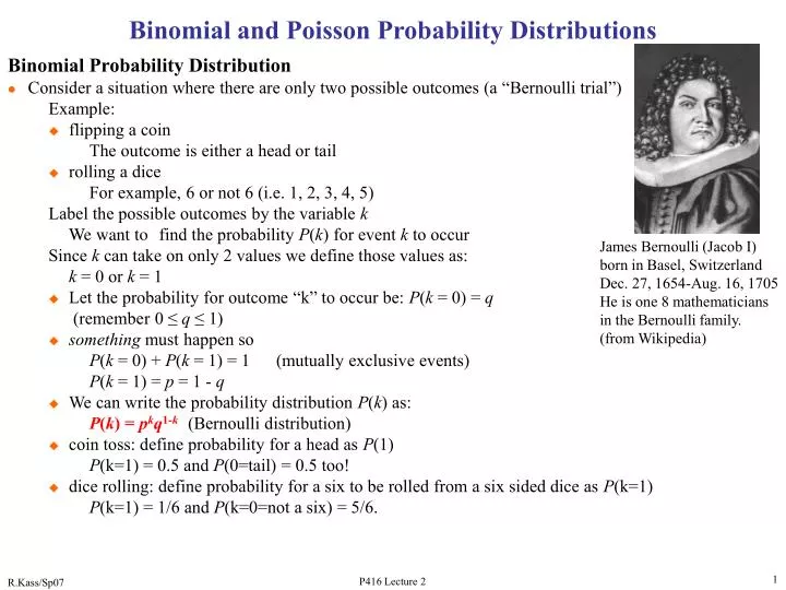
1. Binomial Probability Distribution l Consider a situation where there are only two possible outcomes (a “Bernoulli trial”) Example: u flipping a coin The outcome is either a head or tail u rolling a dice For example, 6 or not 6 (i.e. 1, 2, 3, 4, 5) Label the possible outcomes by the variable k We want tofind the probability P(k) for event k to occur Since k can take on only 2 values we define those values as: k = 0 or k = 1 u Let the probability for outcome “k” to occur be: P(k = 0) = q (remember 0 ≤ q ≤ 1) usomething must happen so P(k = 0) + P(k = 1) = 1 (mutually exclusive events) P(k = 1) = p = 1 - q u We can write the probability distribution P(k) as: P(k) = pkq1-k (Bernoulli distribution) u coin toss: define probability for a head as P(1) P(k=1) = 0.5 and P(0=tail) = 0.5 too! u dice rolling: define probability for a six to be rolled from a six sided dice as P(k=1) P(k=1) = 1/6 and P(k=0=not a six) = 5/6. Binomial and Poisson Probability Distributions James Bernoulli (Jacob I) born in Basel, Switzerland Dec. 27, 1654-Aug. 16, 1705 He is one 8 mathematicians in the Bernoulli family. (from Wikipedia) P416 Lecture 2

2. l What is the mean () of P(k)? l What is the Variance (2) of P(k)? lLet’s do something more complicated: Suppose we have N trials (e.g. we flip a coin N times) what is the probability to get m successes (= heads)? l Consider tossing a coin twice. The possible outcomes are: no heads: P(m = 0) = q2 one head: P(m = 1) = qp + pq (toss 1 is a tail, toss 2 is a head or toss 1 is head, toss 2 is a tail) = 2pq two heads: P(m = 2) = p2 Note: P(m=0)+P(m=1)+P(m=2)=q2+ qp + pq+p2= (p+q)2 = 1 (as it should!) l We want the probability distribution P(m, N, p) where: m = number of success (e.g. number of heads in a coin toss) N = number of trials (e.g. number of coin tosses) p = probability for a success (e.g. 0.5 for a head) Mean and Variance of a discrete distribution (remember p+q=1) we don't care which of the tosses is a head so there are two outcomes that give one head P416 Lecture 2

3. l If we look at the three choices for the coin flip example, each term is of the form: CmpmqN-mm = 0, 1, 2, N = 2 for our example, q = 1 - p always! coefficient Cm takes into account the number of ways an outcome can occur without regard to order. for m = 0 or 2 there is only one way for the outcome (both tosses give heads or tails): C0 = C2 = 1 for m = 1 (one head, two tosses) there are two ways that this can occur: C1 = 2. lBinomial coefficients: number of ways of taking N things m at time 0! = 1! = 1, 2! = 1·2 = 2, 3! = 1·2·3 = 6, m! = 1·2·3···m Order of occurrence is not important u e.g. 2 tosses, one head case (m = 1) n we don't care if toss 1 produced the head or if toss 2 produced the head Unordered groups such as our example are called combinations Ordered arrangements are called permutations For N distinguishable objects, if we want to group them m at a time, the number of permutations: u example: If we tossed a coin twice (N = 2), there are two ways for getting one head (m = 1) u example: Suppose we have 3 balls, one white, one red, and one blue. n Number of possible pairs we could have, keeping track of order is 6 (rw, wr, rb, br, wb, bw): n If order is not important (rw = wr), then the binomial formula gives number of “two color” combinations P416 Lecture 2

4. lBinomial distribution: the probability of m success out of N trials: p is probability of a success and q = 1 - p is probability of a failure l To show that the binomial distribution is properly normalized, use Binomial Theorem: Þ binomial distribution is properly normalized P416 Lecture 2

5. Mean of binomial distribution: A cute way of evaluating the above sum is to take the derivative: Variance of binomial distribution (obtained using similar trick): P416 Lecture 2

6. Example: Suppose you observed m special events (success) in a sample of N events u The measured probability (“efficiency”) for a special event to occur is: What is the error (standard deviation) on the probability ("error on the efficiency"): The sample size (N) should be as large as possible to reduce the uncertainty in the probability measurement. Let’s relate the above result to Lab 2 where we throw darts to measure the value of p. If we inscribe a circle inside a square with side=s then the ratio of the area of the circle to the rectangle is: we will derive this later in the course r s • So, if we throw darts at random at our rectangle then the probability (ºe) of a dart landing inside the • circle is just the ratio of the two areas, p/4. The we can determine p using: p= 4e. The error in p is related to the error in e by: We can estimate how well we can measure p by this method by assuming that e=p/4= (3.14159…)/4: This formula “says” that to improve our estimate of p by a factor of 10 we have to throw 100 (N) times as many darts! Clearly, this is an inefficient way to determine p. P416 Lecture 2

7. Example: Suppose a baseball player's batting average is 0.300 (3 for 10 on average). u Consider the case where the player either gets a hit or makes an out (forget about walks here!). prob. for a hit: p = 0.30 prob. for "no hit”: q = 1 - p = 0.7 u On average how many hits does the player get in 100 at bats? = Np = 100·0.30 = 30 hits u What's the standard deviation for the number of hits in 100 at bats? = (Npq)1/2 = (100·0.30·0.7)1/2 ≈ 4.6 hits we expect ≈ 30 ± 5 hits per 100 at bats u Consider a game where the player bats 4 times: probability of 0/4 = (0.7)4 = 24% probability of 1/4 = [4!/(3!1!)](0.3)1(0.7)3 = 41% probability of 2/4 = [4!/(2!2!)](0.3)2(0.7)2 = 26% probability of 3/4 = [4!/(1!3!)](0.3)3(0.7)1 = 8% probability of 4/4 = [4!/(0!4!)](0.3)4(0.7)0 = 1% probability of getting at least one hit = 1 - P(0) = 1-0.24=76% Pete Rose’s lifetime batting average: 0.303 P416 Lecture 2

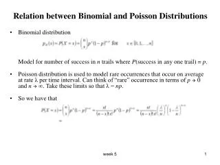
8. Poisson Probability Distribution l The Poisson distribution is a widely used discrete probability distribution. l Consider the following conditions: p is very small and approaches 0 u example: a 100 sided dice instead of a 6 sided dice, p = 1/100 instead of 1/6 u example: a 1000 sided dice, p = 1/1000 N is very large and approaches ∞ example: throwing 100 or 1000 dice instead of 2 dice The product Np is finite l Example: radioactive decay Suppose we have 25 mg of an element very large number of atoms: N ≈ 1020 (avogadro’s number is large!) Suppose the lifetime of this element t = 1012 years ≈ 5x1019 seconds probability of a given nucleus to decay in one second is very small: p = 1/t = 2x10-20/sec BUT Np = 2/sec finite! The number of decays in a time interval is a Poisson process. l Poisson distribution can be derived by taking the appropriate limits of the binomial distribution Siméon Denis Poisson June 21, 1781-April 25, 1840 uradioactive decay unumber of Prussian soldiers kicked to death by horses per year ! uquality control, failure rate predictions N>>m P416 Lecture 2

9. um is always an integer ≥ 0 udoes not have to be an integer It is easy to show that:  = Np = mean of a Poisson distribution 2 = Np =  = variance of a Poisson distribution l Radioactivity example with an average of 2 decays/sec: i) What’s the probability of zero decays in one second? ii) What’s the probability of more than one decay in one second? iii) Estimate the most probable number of decays/sec? u To solve this problem its convenient to maximize lnP(m, ) instead of P(m, ). The mean and variance of a Poisson distribution are the same number! P416 Lecture 2

10. u In order to handle the factorial when take the derivative we use Stirling's Approximation: The most probable value for m is just the average of the distribution u This is only approximate since Stirlings Approximation is only valid for large m. u Strictly speaking m can only take on integer values while  is not restricted to be an integer. If you observed m events in a “counting” experiment, the error on m is ln10!=15.10 10ln10-10=13.03 ®14% ln50!=148.48 50ln50-50=145.60®1.9% P416 Lecture 2

11. Comparison of Binomial and Poisson distributions with mean m = 1 Not much difference between them! N N For N large and m fixed: Binomial Þ Poisson P416 Lecture 2

12. What is a uniform probability distribution: p(x)? p(x)=constant (c) for a £ x £b p(x)=zero everywhere else Therefore p(x1)dx1= p(x2)dx2 if dx1=dx2Þ equal intervals give equal probabilities For a uniform distribution with a=0, b=1 we have p(x)=1 Uniform distribution and Random Numbers 1 p(x) What is a random number generator ? A number picked at random from a uniform distribution with limits [0,1] All major computer languages (FORTRAN, C) come with arandom number generator. FORTRAN: RAN(iseed) The following FORTRAN program generates 5 random numbers: iseed=12345 do I=1,5 y=ran(iseed) type *, y enddo end x 0 1 0.1985246 0.8978736 0.2382888 0.3679854 0.3817045 If we generate “a lot” of random numbers all equal intervals should contain the same amount of numbers. For example: generate: 106 random numbers expect: 105 numbers [0.0, 0.1] 105 numbers [0.45, 0.55] P416 Lecture 2

13. see the fortran tutorial 1234567 FORTRAN statements start in column 7 implicit none character key real count(6), RAN integer i, dice, roll, seed seed = 432211111 10 continue do dice = 1, 6 count(dice) = 0 end do write(6,*)'How many rolls of dice :' read(5,*)roll do i = 1, roll dice = INT(1 + 6*RAN(seed)) count(dice) = count(dice) + 1 end do do i = 1, 6 write(6,*)i, count(i) end do write(6,*) ‘Hit <return> to continue or type q or Q', > ' and <return> to quit the program.' read(5,20)key 20 format(a1) if (key.ne.'q'.and.key.ne.'Q') go to 10 end A Fortran program to throw dice character: variables that are alphanumeric, e.g. A, a, osu real: variables with a decimal point, e.g. 321.45. 0.0567 integer: variables without a decimal point, e.g. 5, 321 seed: an integer variable used by the random number generator RAN A continue statement is a place holder. 10 is the statement number This is a “do loop”. It will repeat 6 times. This question appears on the screen (unit 6) Here you answer the question (unit 5) Another “do loop”. Here we are rolling the dice, using the random number generator. We keep track of the results in the array “count”. Another “do loop”. Here we are writing the results to the monitor screen Allows you to continue the program again or quit If you don’t want to quit then we jump back up to line 10 “end” tells the Fortran compiler that this is the end of the program P416 Lecture 2

14. When we throw an “honest” 6 sided dice we expect each number to appear 1/6 of the time. To simulate this on the computer we want a program that generates the integers [1, 2, 3, 4, 5, 6] in a way that each number is equally likely. DICE=INT(1+6*RAN(ISEED)) RAN(ISEED)Þgives a number [0,1], e.g. 0.33 6*RAN(ISEED)Þ1.98 (multiply by 6) 1+6*RAN(ISEED)Þ2.98 (add 1 to the number) INT(1+6*RAN(ISEED))ÞINTtruncates 2.98 to an integer, 2 As a result of the above code DICE will be equal to “2” We just rolled a “2” How would we roll two dice with a computer? DICE1= INT(1+6*RAN(ISEED)) DICE2= INT(1+6*RAN(ISEED)) TWODI=DICE1+DICE2 The variable TWODI is an integer [2,12] which corresponds to the sum of the numbers on two independent rolls of the dice. Throwing a dice using a computer FORTRAN reads from the right to the left. P416 Lecture 2