Download

1 / 39
440 likes | 766 Views
The Binomial, Poisson, and Normal Distributions. Modified after PowerPoint by Carlos J. Rosas-Anderson. Probability distributions. We use probability distributions because they work –they fit lots of data in real world. Height (cm) of Hypericum cumulicola at Archbold Biological Station.

E N D
The Binomial, Poisson, and Normal Distributions Modified after PowerPoint by Carlos J. Rosas-Anderson
Probability distributions • We use probability distributions because they work –they fit lots of data in real world Height (cm) of Hypericum cumulicola at Archbold Biological Station
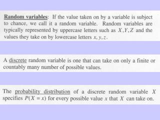
Random variable • The mathematical rule (or function) that assigns a given numerical value to each possible outcome of an experiment in the sample space of interest.
Random variables • Discrete random variables • Continuous random variables
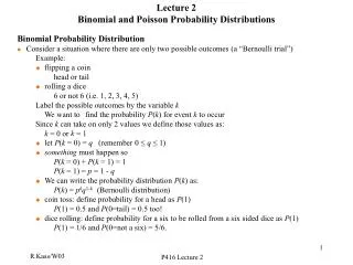
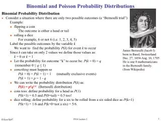
The Binomial DistributionBernoulli Random Variables • Imagine a simple trial with only two possible outcomes • Success (S) • Failure (F) • Examples • Toss of a coin (heads or tails) • Sex of a newborn (male or female) • Survival of an organism in a region (live or die) Jacob Bernoulli (1654-1705)
The Binomial DistributionOverview • Suppose that the probability of success is p • What is the probability of failure? • q = 1 – p • Examples • Toss of a coin (S = head): p = 0.5 q = 0.5 • Roll of a die (S = 1): p = 0.1667 q = 0.8333 • Fertility of a chicken egg (S = fertile): p = 0.8 q = 0.2
The Binomial DistributionOverview • Imagine that a trial is repeated n times • Examples • A coin is tossed 5 times • A die is rolled 25 times • 50 chicken eggs are examined • Assume p remains constant from trial to trial and that the trials are statistically independent of each other
The Binomial DistributionOverview • What is the probability of obtaining x successes in n trials? • Example • What is the probability of obtaining 2 heads from a coin that was tossed 5 times? P(HHTTT) = (1/2)5 = 1/32
The Binomial DistributionOverview • But there are more possibilities: HHTTT HTHTT HTTHT HTTTH THHTT THTHT THTTH TTHHT TTHTH TTTHH P(2 heads) = 10 × 1/32 = 10/32
The Binomial DistributionOverview • In general, if trials result in a series of success and failures, FFSFFFFSFSFSSFFFFFSF… Then the probability of x successes in that order is P(x) = q q p q = px qn – x
n! n! x!(n – x)! x!(n – x)! The Binomial DistributionOverview • However, if order is not important, then where is the number of ways to obtain x successes in n trials, and i! = i (i – 1) (i – 2) … 2 1 P(x) = px qn – x
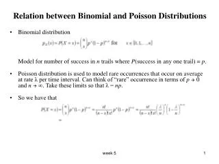
The Poisson DistributionOverview • When there is a large number of trials, but a small probability of success, binomial calculation becomes impractical • Example: Number of deaths from horse kicks in the Army in different years • The mean number of successes from n trials is µ = np • Example: 64 deaths in 20 years from thousands of soldiers Simeon D. Poisson (1781-1840)
e -µµx P(x) = x! The Poisson DistributionOverview • If we substitute µ/n for p, and let n tend to infinity, the binomial distribution becomes the Poisson distribution:
The Poisson DistributionOverview • Poisson distribution is applied where random events in space or time are expected to occur • Deviation from Poisson distribution may indicate some degree of non-randomness in the events under study • Investigation of cause may be of interest
The Poisson DistributionEmission of -particles • Rutherford, Geiger, and Bateman (1910) counted the number of -particles emitted by a film of polonium in 2608 successive intervals of one-eighth of a minute • What is n? • What is p? • Do their data follow a Poisson distribution?
e -3.87(3.87)x 2680 P(x) = 2608 x! The Poisson DistributionEmission of -particles • Calculation of µ: µ = No. of particles per interval = 10097/2608 = 3.87 • Expected values:
Random events Regular events Clumped events The Poisson DistributionEmission of -particles
The closed unit interval, which contains all numbers between 0 and 1, including the two end points 0 and 1 Uniform random variables Subinterval [5,6] Subinterval [3,4] The probability density function
The Expected Value of a continuous Random Variable For an uniform random variable x, where f(x) is defined on the interval [a,b], and where a<b, and
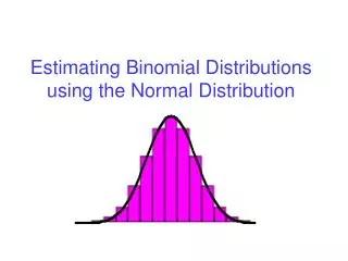
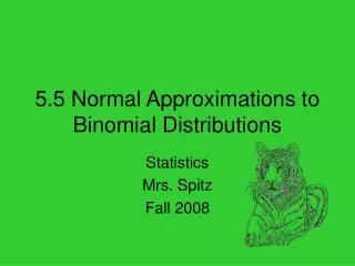
The Normal DistributionOverview • Discovered in 1733 by de Moivre as an approximation to the binomial distribution when the number of trails is large • Derived in 1809 by Gauss • Importance lies in the Central Limit Theorem, which states that the sum of a large number of independent random variables (binomial, Poisson, etc.) will approximate a normal distribution • Example: Human height is determined by a large number of factors, both genetic and environmental, which are additive in their effects. Thus, it follows a normal distribution. Abraham de Moivre (1667-1754) Karl F. Gauss (1777-1855)
1 (x)2/22 f (x) = e 2 x2 x1 The Normal DistributionOverview • A continuous random variable is said to be normally distributed with mean and variance 2 if its probability density function is • f(x) is not the same as P(x) • P(x) would be 0 for every x because the normal distribution is continuous • However, P(x1 < X ≤ x2) = f(x)dx
The Normal DistributionOverview Mean changes Variance changes
The Normal DistributionLength of Fish • A sample of rock cod in Monterey Bay suggests that the mean length of these fish is = 30 in. and 2 = 4 in. • Assume that the length of rock cod is a normal random variable • If we catch one of these fish in Monterey Bay, • What is the probability that it will be at least 31 in. long? • That it will be no more than 32 in. long? • That its length will be between 26 and 29 inches?
The Normal DistributionLength of Fish • What is the probability that it will be at least 31 in. long?
The Normal DistributionLength of Fish • That it will be no more than 32 in. long?
The Normal DistributionLength of Fish • That its length will be between 26 and 29 inches?
Standard Normal Distribution • μ=0 and σ2=1
Useful properties of the normal distribution • The normal distribution has useful properties: • Can be added E(X+Y)= E(X)+E(Y) and σ2(X+Y)= σ2(X)+ σ2(Y) • Can be transformed with shift and change of scale operations
Consider two random variables X and Y Let X~N(μ,σ) and let Y=aX+b where a and b area constants Change of scale is the operation of multiplying X by a constant “a” because one unit of X becomes “a” units of Y. Shift is the operation of adding a constant “b” to X because we simply move our random variable X “b” units along the x-axis. If X is a normal random variable, then the new random variable Y created by this operations on X is also a random normal variable
For X~N(μ,σ) and Y=aX+b • E(Y) =aμ+b • σ2(Y)=a2σ2 • A special case of a change of scale and shift operation in which a = 1/σ and b =-1(μ/σ) • Y=(1/σ)X-μ/σ • Y=(X-μ)/σ gives • E(Y)=0 and σ2(Y) =1
The Central Limit Theorem • That Standardizing any random variable that itself is a sum or average of a set of independent random variables results in a new random variable that is nearly the same as a standard normal one. • The only caveats are that the sample size must be large enough and that the observations themselves must be independent and all drawn from a distribution with common expectation and variance.
Exercise Location of the measurement