Download
1 / 25
250 likes | 574 Views
The Normal, Binomial, and Poisson Distributions. Engineering Experimental Design Winter 2003. In Today’s Lecture. What the normal, binomial, and Poisson distributions look like What parameters describe their shapes How these distributions can be useful. The Normal Distribution.

E N D
The Normal, Binomial, and Poisson Distributions Engineering Experimental Design Winter 2003
In Today’s Lecture . . . • What the normal, binomial, and Poisson distributions look like • What parameters describe their shapes • How these distributions can be useful
The Normal Distribution • Also called a “Gaussian” distribution or a bell-shaped curve • Centered around the mean with a width determined by the standard deviation • Total area under the curve = 1.0 • f(x) = (1/ sqrt(2)) exp(-(x-)/(22))
To Draw a Normal Distribution . . . • For a mean of 5 and a standard deviation of 1: mu = 5; % set mean sigma = 1; % set standard deviation x = [0 : 0.1 : 10]; % define x-axis y = normpdf(x,mu,sigma); plot(x,y);
What Does a Normal Distribution Describe? • Imagine that you go to the lab and very carefully measure out 5 ml of liquid and weigh it. • Imagine repeating this process many times. • You won’t get the same answer every time, but if you make a lot of measurements, a histogram of your measurements will approach the appearance of a normal distribution.
What Does a Normal Distribution Describe? • Imagine that you hold a ping pong ball over a target on the floor, drop it, and record the distance between where it fell and the center of the target. • Imagine repeating this process many times. • You won’t get the same distance every time, but if you make a lot of measurements, the histogram of your measurements will approach a normal distribution.
What Does a Normal Distribution Describe? • Any situation in which the exact value of a continuous variable is altered randomly from trial to trial. • The random uncertainty or random error • Note: If your measurement is biased (e.g., the scale is off or there is a steady wind blowing the ping pong ball), then your measurements can be normally distributed around some value other than the true value or target.
How Do You Use The Normal Distribution? • You don’t • Use the area UNDER the normal distribution • For example, the area under the curve between x=a and x=b is the probability that your next measurement of x will fall between a and b
How Do You Get and ? • To draw a normal distribution (and integrate to find the area under it), you must know and f(x) = (1/ sqrt(2)) exp(-(x-)/(22)) • If you made an infinite number of measurements, their mean would be and their standard deviation would be In practice, you have a finite number of measurements with mean x and standard deviation s • For now, and will be given Later we’ll use x and s to estimate and This x is written in your book as an x with a line over it
The Standard Normal Distribution • It is tedious to integrate a new normal distribution for every single measurement, so use a “standard normal distribution” with tabulated areas. • Convert your measurement x to a standard score z = (x - ) / • Use the standard normal distribution = 0 and = 1 areas tabulated in front of text
Example • Historical data shows that the temperature of a particular pipe in a continuous production line is (94 ± 5)°C (±1). You glance at the control display and see that T = 87 °C. How abnormal is this measurement?
Example • Historical data shows that the temperature of a particular pipe in a normally-operating continuous production line is (94 ± 5)°C (±1). You glance at the control display and see that T = 87 °C. How abnormal is this measurement? z = (87 – 94)/5 = -1.4 From the table in the front of the text, -1.4 gives an area of 0.0808. In other words, when the line is operating normally, you would expect to see even lower temperatures about 8 % of the time. This measurement alone should not worry you.
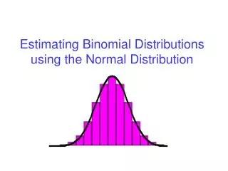
What Does the Binomial Distribution Describe? • The probability of getting all “tails” if you throw a coin three times • The probability of getting four “2s” if you roll six dice • The probability of getting all male puppies in a litter of 8 • The probability of getting two defective batteries in a package of six
The Binomial Distribution • p(x) = (n!/(x!(n-x)!))x(1-)n-x • The probability of getting the result of interest x times out of n, if the overall probability of the result is • Note that here, x is a discrete variable • Integer values only • In a normal distribution, x is a continuous variable This is NOT 3.14159!
Uses of the Binomial Distribution • Quality assurance • Genetics • Experimental design
To Draw a Binomial Distribution • n = 6; % number of dice rolled • pi = 1/6; % probability of rolling a 2 on any die • x = [0 1 2 3 4 5 6]; % # of 2s out of 6 • y = binopdf(x,n,pi); • bar(x,y)
To Draw a Binomial Distribution • n = 8; % number of puppies in litter • pi = 1/2; % probability of any pup being male • x = [0 1 2 3 4 5 6 7 8]; % # of males out of 8 • y = binopdf(x,n,pi); • bar(x,y)
The Shape of the Binomial Distribution • Shape is determined by values of n and • Only truly symmetric if = 0.5 • Approaches normal distribution if n is large, unless is very small • Mean number of “successes” is n • Standard deviation of distribution is sqrt(n (1- ))
Example • While you are in the bathroom, your little brother claims to have rolled a “Yahtzee” (5 matching dice out of five) in one roll of the five dice. How justified would you be in beating him up for cheating?
Example • While you are in the bathroom, your little brother claims to have rolled a “Yahtzee” (5 matching dice out of five) in one roll of the five dice. How justified would you be in beating him up for cheating? • n = 5, = 1/6, x = 5 • p(x) = (5!/(x!(0)!))(1/6)5(5/6)0 or • p = binopdf(5,5,1/6) = 1.29 10-4 • In other words, the chances of this happening are 1 / 7750.
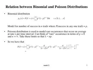
The Poisson Distribution • Probability of an event occurring x times in a particular time period • p(x) = xe- / x! • = average number of events expected during time period determines shape of distribution • The binomial distribution approaches the Poisson distribution if n is large and small
Example • A production line produces 600 parts per hour with an average of 5 defective parts an hour. If you test every part that comes off the line in 15 minutes, what are your chances of finding no defective parts (and incorrectly concluding that your process is perfect)?
Example • A production line produces 600 parts per hour with an average of 5 defective parts an hour. If you test every part that comes off the line in 15 minutes, what are your chances of finding no defective parts (and incorrectly concluding that your process is perfect)? • = (5 parts/hour)*(0.25 hours observed) = 1.25 parts • x = 0 • p(0) = e-1.25(1.25)0 / 0! = e-5 = 0.297 or about 29 %
To Draw a Poisson Distribution • lambda = 1.25; % average defects in 15 min • x = [0 1 2 3 4 5]; % number observed • y = poisspdf(x,lambda); • bar(x,y)
Example • A production line produces 600 parts per hour with an average of 5 defective parts an hour. If you test every part that comes off the line in 15 minutes, what are your chances of finding no defective parts (and incorrectly concluding that your process is perfect)? • Why not the binomial distribution? n = 600 / 4 = 150 ------ large • = 5 / 600 = 0.008 ------ small You don’t want to calculate 150!