Hydrodynamics: Viscosity and Diffusion
Hydrodynamics: Viscosity and Diffusion. Hydrodynamics is the study of mechanics in a liquid, where the frictional drag of the liquid cannot be ignored First let’s just consider fluid flow, where the fluid (e.g., water) is treated as continuous.

Hydrodynamics: Viscosity and Diffusion
E N D
Presentation Transcript
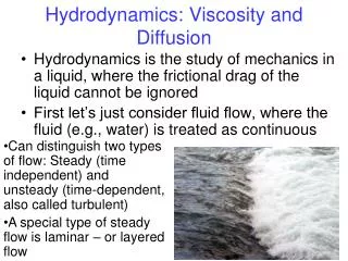
Hydrodynamics: Viscosity and Diffusion • Hydrodynamics is the study of mechanics in a liquid, where the frictional drag of the liquid cannot be ignored • First let’s just consider fluid flow, where the fluid (e.g., water) is treated as continuous • Can distinguish two types of flow: Steady (time independent) and unsteady (time-dependent, also called turbulent) • A special type of steady flow is laminar – or layered flow
Reynolds Number • R = ruL/h, where u and L are the velocity and length of the object, and r and h are the density and viscosity of the fluid • All macromolecules/bacteria/viruses are in the low R regime where viscous forces dominate • When modeling the flow of a fluid (water) around such a microscopic object, it is important to consider the boundary layer of fluid near the object – or, its hydration layer • In physics, the two limits are “stick” and “slip” boundary conditions – with stick conditions appropriate for macromolecules
Hydrodynamic Flow experiments • A number of experimental techniques involve forcing a macromolecule through a fluid (external force can be electric, gravity, hydrodynamic, or even magnetic) • In this case we have: where f is the friction coefficient. • After an extremely short time (~ ps), these two forces balance and the acceleration goes to zero so that
Friction coefficient • Stokes derived the friction coefficient for a sphere (w/ stick BC): where R is the sphere radius • For a few other shaped objects there are closed expressions for f, but f for a sphere is the minimum value for an equal volume (since f depends mostly on surface area contact with the fluid and a sphere has the minimum surface area for objects of the same volume) • Rods - f depends on L and axial ratio – Broersma story • There are now computer modeling programs that treat any shaped object as a collection of spheres and can calculate f IgG lysozyme
Concentration effects on f • Stokes law is valid only in the limit of low concentration where individual spheres do not “see” each other • At higher concentrations, flow “wakes” interact with other spheres and increase the friction coefficient, so that to a first approximation:
Viscosity of pure fluid • Definition for laminar flow: shear stress = F/A (tangential force/area) velocity gradient = du/dy = rate of strain Shear stress = ho (rate of strain) – or F/A = ηo(du/dy) - defines a Newtonian fluid ηunits are dyne-s/cm2 = 1 Poise or 1 N-s/m2 = 10 Poise hwater = 1 cP at 20oC
Viscous Flow in a cylinder • Laminar flow – velocity profile: • Flow rate = Volume/time = Q = (pPR4/8hL) (Poiseuille’s law, 1835; French physician, blood flow) • Measuring h: Q ~ P/h (R,L fixed) and P=rgL so time ~ h/r Then with a standard (water?) Ostwald viscometer
Viscosity of Solutions of Macromolecules • Macromolecules distort flow, leading to increased viscosity. Einstein (1906) first solved this problem for spheres: with n = 2.5 for spheres and whereF is the volume fraction occupied by the macromolecules. • For other shapes the coefficient, n, is larger than 2.5 • Other expressions: relative viscosity = hrel = h/ho or specific viscosity = hspec = (h-ho)/ho = hrel – 1 = nF
Intrinsic Viscosity • Now, F = volume of macromolecule/cm3, but this is equal to , where the partial specific volume is (volume/gm macro) and the concentration is (gm/cm3) • So, we have , which when extrapolated to c = 0 defines the intrinsic viscosity
Measuring Macromolecular Viscosity • Need low stress, low concentration – • Older method: Ubbelohde glass viscometer • Newer methods: • Couette viscometer • Stress rheometer
Example of use of Viscosity Data • First evidence for circular DNA (in T2) h A C B time Add pancreatic DNAase- induces ss breaks A single nicks B ds breaks h decreases C first cut leads to h increase, then decrease
F=ma in Diffusion • F(t) = random fluctuating force from solvent collisions(~1016/s at room T for a 1 mm sphere) • We don’t care about details, but want <time averages> <xF(t)> - f<xu(t)> = m <x a> but <xF> = 0 so now, let y = x2 and note that So we get Equipartition of energy says (from thermo, with kB = 1.38x10⁻²³J/K): <KE> = ½ kBT or then
Particle Diffusion • Solution to this is: <y> = (2kBT/f)t = <x2> A result due to A. Einstein (1905) • So, <x> = 0, but <x2> = 2Dt, where D = kBT/f • In 3-D, since r2 = x2 + y2 + z2 and <x2>=<y2>=<z2>, we have <r2>=6Dt Twenty seconds of a measured random walk trajectory for a micrometer-sized ellipsoid undergoing Brownian motion in water. The ellipsoid orientation, labeled with rainbow colors, illustrates the coupling of orientation and displacement and shows clearly that the ellipsoid diffuses faster along its long axis compared to its short axis.
Second Approach to Diffusion • Instead of looking at a single particle, we can consider the concentration c(x, y, z) • If we start with a non-uniform initial concentration profile, diffusion tends to randomize leading to a uniform c • In 1-D first, introduce the particle flux = J = #/area/time Can show J = cu, where c = #/volume [# = cAL, but u=L/t, so J=cAL/(At)=cu] • Fick’s First Law says J=-D[dc/dx] ; flow ~ c variation (also holds for heat-T, fluid-P, electric current-potential) L A
Diffusion Equation • But J varies with x and t: or • Combining this with Fick’s First law, we get the diffusion eqution: J(x) J(x+dx) x x+dx
Two Solutions to the Diffusion Eqn. • Solutions depend on initial conditions • Narrow band of c at time zero • See Figure D3.7 for step gradient initial condition c Time 0 – very sharply peaked x x=0 c x x=0
Two complications due to Particle Interactions • Excluded volume: particles occupy some volume • Concentration dependence of f: Combining these results in: Note: If c is expressed as a volume fraction, F (with ) then for spheres A = 8 and A’ = 6.5
Why not always work at very low c? • Some systems are only interesting, or interact, at higher c • Need a probe to measure c(x,t): light, radioactive tracer, fluorescence, etc., and need some threshold signal to detect • Some molecules fall apart at very low c – or even denature – e.g. myosin, hemoglobin
Temperature and Solvent Effects • Remember with both T (K) and η varying with temperature; η varies about 2% per oC for water near 20oC • With a solvent that includes salts (changing viscosity) we have • Also, remember that for equivalent sphere f=6phR, with R = hydrodynamic radius, including hydration
How to Measure D • Spreading Boundary Method – used in ultracentrifuge (see Figure D3.7 again) • FRAP (Fluorescence Recovery After Photobleaching) – • DLS (Dynamic Light Scattering) – more later • NMR (Nuclear Magnetic Resonance) – for small molecules only – later Typical D values are ~10-7 cm2/s for small proteins to ~10-9 cm2/s for large ones