Download
1 / 59
590 likes | 710 Views
Explore review of search strategies, including uninformed and iterative deepening search, with focus on state space, completeness, optimality, time, and space complexity. Learn about breadth-first, depth-first, and uniform-cost searches and their implementations. Discover properties and benefits of each strategy.

E N D
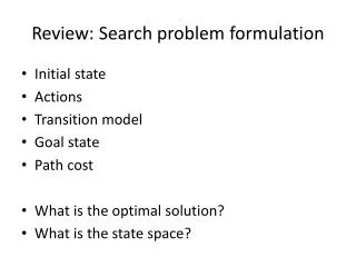
Review: Search problem formulation • Initial state • Actions • Transition model • Goal state • Path cost • What is the optimal solution? • What is the state space?
Review: Tree search • Initializethe fringe using the starting state • While the fringe is not empty • Choose a fringe node to expand according to search strategy • If the node contains the goal state, return solution • Else expand the node and add its children to the fringe
Search strategies • A search strategy is defined by picking the order of node expansion • Strategies are evaluated along the following dimensions: • Completeness:does it always find a solution if one exists? • Optimality:does it always find a least-cost solution? • Time complexity:number of nodes generated • Space complexity: maximum number of nodes in memory • Time and space complexity are measured in terms of • b: maximum branching factor of the search tree • d: depth of the optimal solution • m: maximum length of any path in the state space (may be infinite)
Uninformed search strategies • Uninformed search strategies use only the information available in the problem definition • Breadth-first search • Uniform-cost search • Depth-first search • Iterative deepening search
Breadth-first search • Expand shallowest unexpanded node • Implementation: • fringe is a FIFO queue, i.e., new successors go at end A B C D E F G
Breadth-first search • Expand shallowest unexpanded node • Implementation: • fringe is a FIFO queue, i.e., new successors go at end A B C D E F G
Breadth-first search • Expand shallowest unexpanded node • Implementation: • fringe is a FIFO queue, i.e., new successors go at end A B C D E F G
Breadth-first search • Expand shallowest unexpanded node • Implementation: • fringe is a FIFO queue, i.e., new successors go at end A B C D E F G
Breadth-first search • Expand shallowest unexpanded node • Implementation: • fringe is a FIFO queue, i.e., new successors go at end A B C D E F G
Properties of breadth-first search • Complete? Yes (if branching factor bis finite) • Optimal? Yes – if cost = 1 per step • Time? Number of nodes in a b-ary tree of depth d: O(bd) (d is the depth of the optimal solution) • Space? O(bd) • Space is the bigger problem (more than time)
Uniform-cost search • Expand least-cost unexpanded node • Implementation: fringe is a queue ordered by path cost (priority queue) • Equivalent to breadth-first if step costs all equal • Complete? Yes, if step cost is greater than some positive constant ε • Optimal? Yes – nodes expanded in increasing order of path cost • Time? Number of nodes with path cost≤ cost of optimal solution (C*), O(bC*/ ε) This can be greater than O(bd): the search can explore long paths consisting of small steps before exploring shorter paths consisting of larger steps • Space? O(bC*/ ε)
Depth-first search • Expand deepest unexpanded node • Implementation: • fringe = LIFO queue, i.e., put successors at front A B C D E F G
Depth-first search • Expand deepest unexpanded node • Implementation: • fringe = LIFO queue, i.e., put successors at front A B C D E F G
Depth-first search • Expand deepest unexpanded node • Implementation: • fringe = LIFO queue, i.e., put successors at front A B C D E F G
Depth-first search • Expand deepest unexpanded node • Implementation: • fringe = LIFO queue, i.e., put successors at front A B C D E F G
Depth-first search • Expand deepest unexpanded node • Implementation: • fringe = LIFO queue, i.e., put successors at front A B C D E F G
Depth-first search • Expand deepest unexpanded node • Implementation: • fringe = LIFO queue, i.e., put successors at front A B C D E F G
Depth-first search • Expand deepest unexpanded node • Implementation: • fringe = LIFO queue, i.e., put successors at front A B C D E F G
Depth-first search • Expand deepest unexpanded node • Implementation: • fringe = LIFO queue, i.e., put successors at front A B C D E F G
Depth-first search • Expand deepest unexpanded node • Implementation: • fringe = LIFO queue, i.e., put successors at front A B C D E F G
Properties of depth-first search • Complete? Fails in infinite-depth spaces, spaces with loops Modify to avoid repeated states along path complete in finite spaces • Optimal? No – returns the first solution it finds • Time? Could be the time to reach a solution at maximum depth m: O(bm) Terrible if m is much larger than d But if there are lots of solutions, may be much faster than BFS • Space? O(bm), i.e., linear space!
Iterative deepening search • Use DFS as a subroutine • Check the root • Do a DFS searching for a path of length 1 • If there is no path of length 1, do a DFS searching for a path of length 2 • If there is no path of length 2, do a DFS searching for a path of length 3…
Properties of iterative deepening search • Complete? Yes • Optimal? Yes, if step cost = 1 • Time? (d+1)b0 + d b1 + (d-1)b2 + … + bd = O(bd) • Space? O(bd)
Informed search • Idea: give the algorithm “hints” about the desirability of different states • Use an evaluation function to rank nodes and select the most promising one for expansion • Greedy best-first search • A* search
Heuristic function • Heuristic function h(n) estimates the cost of reaching goal from node n • Example: Start state Goal state
Greedy best-first search • Expand the node that has the lowest value of the heuristic function h(n)
Properties of greedy best-first search • Complete? No – can get stuck in loops start goal
Properties of greedy best-first search • Complete? No – can get stuck in loops • Optimal? No
Properties of greedy best-first search • Complete? No – can get stuck in loops • Optimal? No • Time? Worst case: O(bm) Best case: O(bd) – If h(n) is 100% accurate • Space? Worst case: O(bm)
A* search • Idea: avoid expanding paths that are already expensive • The evaluation function f(n) is the estimated total cost of the path through node n to the goal: f(n) = g(n) + h(n) g(n): cost so far to reach n (path cost) h(n): estimated cost from n to goal (heuristic)
Admissible heuristics • A heuristic h(n) is admissible if for every node n, h(n)≤ h*(n), where h*(n) is the true cost to reach the goal state from n • An admissible heuristic never overestimates the cost to reach the goal, i.e., it is optimistic • Example: straight line distance never overestimates the actual road distance • Theorem: If h(n)is admissible, A*is optimal
Optimality of A* • Proof by contradiction • Let n* be an optimal goal state, i.e., f(n*) = C* • Suppose a solution node n with f(n) > C* is about to be expanded • Let n' be a node in the fringe that is on the path to n* • We have f(n') = g(n') + h(n') ≤C* • But then, n' should be expanded before n – a contradiction n' n* n
Optimality of A* • In other words: • Suppose A* terminates its search at n* • It has found a path whose actual costf(n*) = g(n*) is lower than the estimated costf(n) of any path going through any fringe node • Since f(n) is an optimistic estimate, there is no way n can have a successor goal state n’ with g(n’) < C* f(n*) = C* n* n f(n) > C* g(n') f(n) > C* n'
Optimality of A* • A* is optimally efficient – no other tree-based algorithm that uses the same heuristic can expand fewer nodes and still be guaranteed to find the optimal solution • Any algorithm that does not expand all nodes with f(n) < C* risks missing the optimal solution