Abstract

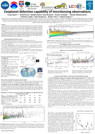
1. Maximizing planet detection zone area Microlensing isunique in its sensitivity to wider-orbit (i.e. cool) planetary-mass bodies. Based on the approach presented in [1], at each time step for different events we calculate the detection zone area and the probability of detection of an exoplanet. The event with a maximum probability at a time step is chosen for observations. We define the ‘detection zone’ as the region on the lens plane (x,y) where the light curve anomaly δ(t,x,y,q) is large enough to be detected by the observations (q is the ratio of the planet to that of the star). The photometric S/N (signal to noise) ratio and hence the area w of an isolated planet detection zone scales as the square root of the exposure time : S/N = (Δt /τ) 1/2, w = g Δt 1/2 . Here τ is the exposure time required to reach S/N=1. The 'goodness' gi of an available target depends on the target's brightness and magnification, the telescope and detector characteristics, and observing conditions (air mass, sky brightness, seeing). See [1] for details. [1] Horne K., Snodgrass C., Tsapras Y., MNRAS, 2009, v. 396, 2087-2102. Seeing (in arcsec) vs. air mass. FTS observations of 39 events. A thick straight line is based on χ2 optimization (y= so + s1(x-1), so =1.334, s1=0.519). Thinner straight lines differ from this line by +/- Ϭ (Ϭ=0.367). Non-straight lines show mean and median values (the line for the mean value is thicker). Sky brightness residuals vs. solar elevation The influence of solar elevation θSun on sky brightness began to play a role at θSun>-14o, and was considerable at θSun>-7o. For example, if we consider only FTS observations with the Moon below the horizon, then sky brightness residual sbr can be up to -3 mag at -8o<θSun<-7o, sbr>-1 mag at θSun<-8o, and sbr>-0.4 mag at θSun<-14o. Light curves for events selected for observations Exoplanet detection capability of microlensing observationsSergei Ipatov1,2, Keith Horne3, Khalid Alsubai4, Dan Bramich5, Martin  Dominik3,*, Markus Hundertmark3, Christine Liebig3, Colin Snodgrass6,   Rachel Street7, Yiannis Tsapras7,81) Alsubai Est. for Scientific Studies, Doha, Qatar; 2) Vernadsky Institute, Moscow, Russia; 3) Univ. of St. Andrews, St. Andrews, Scotland, United Kingdom; 4) Qatar Foundation, Doha, Qatar; 5) European Southern Observatory, Garching bei München, Germany; 6) Max Planck Institute for Solar System Research, Katlenburg-Lindau, Germany; 7) Las Cumbres Observatory Global Telescope Network, Santa Barbara, USA; 8) School of Physics and Astronomy, Queen Mary, University of London, United Kingdom. * Royal Society University Research Fellow. †supported by Qatar National Research Fund (QNRF), member of Qatar Foundation (grant NPRP 09-476-1-078) Telescopes (with numbers Ntfrom 1 to 13) considered: • 1. 2m FTS - Faulkes Telescope South - Siding Springs, Australia. • 2. 2m FTN - Faulkes Telescope North - Haleakela, Hawaii. • 3. 2m LT - Liverpool Telescope - La Palma, Canary Islands. • 4. 1.3m OGLE - The Optical Gravitational Lensing Experiment - Las Campanas, Chile • 5-7. Three 1m CTIO - Cerro Tololo Inter-American Observatory in Chile . • 8. 1m MDO - McDonald observatory in Texas. • 9-11. Three 1m SAAO - South African Astronomical Observatory. • 12-13. Two 1m SSO - Siding Spring Observatory near Coonabarabran, New South Wales, Australia. Light curves (with error bars) for events selected for observations with OGLE (at actual times of peaks of light curves). Considered events: 110001-111562. Time intervals for events selected for observations with OGLE (at actual times of peaks of light curves). Considered events: 1110001-111562. Comparison of the efficiency of telescopes for microlensing observations Our simulator suggests what events it is better to observe at specific time intervals with a specific telescope in order to increase the probability of finding new exoplanets using microlensing observations. For estimates of the probability, for best events we considered wsum=∑ gi[(Δt+tdone)1/2-tdone1/2] (where Δt=2tslew for an event observed at a current time, and Δt=tslew and tdone=0 for other events) and rwsumt=(wsum/wsumOGLE)×(tsum/tsumOGLE), where tsum is the total time during considered time interval when it is possible to observe at least one event. For best events we also calculated wsumo=∑gi[(ts+tdone)1/2-tdone1/2] andrwsumto=(wsumo/wsumoOGLE)×(tsum/tsumOGLE) with ts=20 s. The value of tsum/tsumOGLE is about 0.65, 0.55, and 0.52 for FTN, LT, and MDO, respectively. For other considered sites, it is close to 1. In our calculations, rwsumtand rwsumto for observations with a 1-m telescope (located at CTIO, SAAO, SSO, or MDO) equipped with the Sinistro CCD, and with a 2-m telescope (FTS, FTN, or LT) were mainly about 0.8-1.2 and 1.4-2.2 of that for OGLE, respectively. The above ratio of probabilities is different for different considered events, and can be outside the above intervals (see the plot below). The ratio of wsum for FTS and SSO located at the same site usually was about 2. For the SBIG CCD, the values of wsum (and wsumo) were smaller by a factor of ~1.2 than those for the Sinistro CCD. In the case when 1-m telescopes located at the same site observe different events at the same time, the values of wsum usually are relatively close for different telescopes if there are no high light curve peaks during (or close to) the considered time intervals, and wsum can differ much for the telescopes in the case of the high peaks. In the latter case, it may be better to observe the same event with all telescopes, even though in this case a detection zone area grows as a square root of an effective area of telescopes (i.e., sqrt of the number of 1-m telescopes used). The value of wsum was typically proportional to the diameter of the mirror. The difference in wsum is about 5% if for SSO we use the values of Isky(0) and the dependence of seeing vs. air mass as those for OGLE, compared to those for FTS. The values of wsum obtained at our approach are close to those obtained for the choice of events selected for observations according to [3] Dominik et al., Astron. Nachr, 2010, v. 331, No 7, 671-691. If only events with the peak value of the magnification Amax>50 (4% of events) are observed, then the ratio r50 of the value of wsum for such observations to the value of wsum for the observations allowed for all 1562 events can differ by an order of magnitude for different considered time intervals. For example, for OGLE r50 equals 0.07 and 0.99 for 5-day intervals starting from April 22 and August 1, 2011, respectively; for 100-day intervals, r50 is 0.63 and 0.83, respectively. ------------------------------------------------------------------------------------------------------------------------------------------ • Observations analyzed for construction of sky model: • For studies of sky brightness for FTS, FTN, and LT, we considered those events observed in 2011 for which .dat files are greater than 1 kbt (i.e., the minimum number of lightcurve data points is greater than 15): FTS - 39 events; FTN - 19 events, LT – 20 events. For OGLE we considered 20 events (110251-110270). • Calculations of Isky(0) (sky brightness at zenith)and the coefficients (k1 and ko) presented in the tables and on the plots were based on χ2 optimization of the straight line fit (y=k1·x+ko, χ2=∑[(yi-k1·xi-ko)/σi]2, σi2 is variance). The value of Isky(0)was chosen in such a way that the sum of squares of differences between observational and model sky brightness magnitudes were minimum in the case when the Moon is below the horizon. The used sky model was based mainly on [2] K. Krisciunas & B. Schaefer, PASP, 1991, v. 103, 1033-1039. Abstract We summarize the status of a computer simulator for microlens planet surveys. The simulator generates synthetic light curves of microlensing events observed with specified networks of telescopes over specified periods of time. The main purpose is to assess the impact on planet detection capabilities of different observing strategies, and different telescope resources, and to quantify the planet detection efficiency of our actual observing network, so that we can use the observations to constrain planet abundance distributions. We have developed models for sky brightness and seeing, calibrated by fitting to data from the OGLE survey and RoboNet observations in 2011. Time intervals during which events are observable are identified by accounting for positions of the Sun, the Moon and other restrictions on telescope pointing. Simulated observations are then generated for an algorithm that adjusts target priorities in real time with the aim of maximizing planet detection zone area summed over all the available events. The exoplanet detection capability of microlensing observations is compared for several telescopes. Dependences of seeing on air mass and values of sky brightness at zenith obtained based on analysis of observations Values Isky(0) of sky brightness at zenith (I magnitude per square arcsec) for an extinction coefficient extmag=0.05 (for extmag equal to 0 and 0.1, values of Isky(0) differed by less than 0.3%). Seeing (FWHM in arcsec) vs. airmass (χ2 approximation): seeing=so +s1×(airmass-1) The values of rwsumt=(wsum/wsumOGLE)/(tsum/tsumOGLE), which characterize the exoplanet detection capability of observations (in the case of 1562 events available for observations), vs. the numberNt of a telescope in the case when 1 m telescopes (equipped with the Sinistro CCD) located at the same site observe different events at the same time. Black or red crests and ellipses are for the 100-day time interval beginning from April 22 and August 1, 2011, respectively. The signs for calculations with actual values of t0 (the time corresponding to the peak of a light curve) andwith random values of t0 (t0 = RNDM∙(tmx+2tE )-tE+to, where tE is the time scale equal to the ratio of the angular Einstein radius to the relative proper motion, RNDM is a random value between 0 and 1, tmx is the duration of the considered time interval, to is the beginning of the interval) are black greater and red smaller, respectively. Green crests are for actual values of t0 and 90-day interval beginning from April 22, 2011. Small signs are for non-priority telescopes. For random values of t0, the number of light curve peaks was greater. . Sky brightness (mag) vs. air mass for the Moon below the horizon. Different points are for OGLE observations of 20 different events. The lines are for the χ2 optimization (b=b1·a+bo) with different bo (different values for different events) and the same b1. The most solid line is for the model for which bois the same for all events. For the Moon below the horizon, the values of bo (which characterize sky zenith brightness near different events) differ typically by not more that 1 mag. Contact: siipatov@hotmail.com