Download
1 / 64
640 likes | 667 Views
Discover how rewrite rules are instrumental in various system resolving techniques such as resolution and demodulation, with a focus on ACL2. Learn about formal foundations, performance considerations, and the application of rewrite rules in algorithmic decision-making processes.

E N D
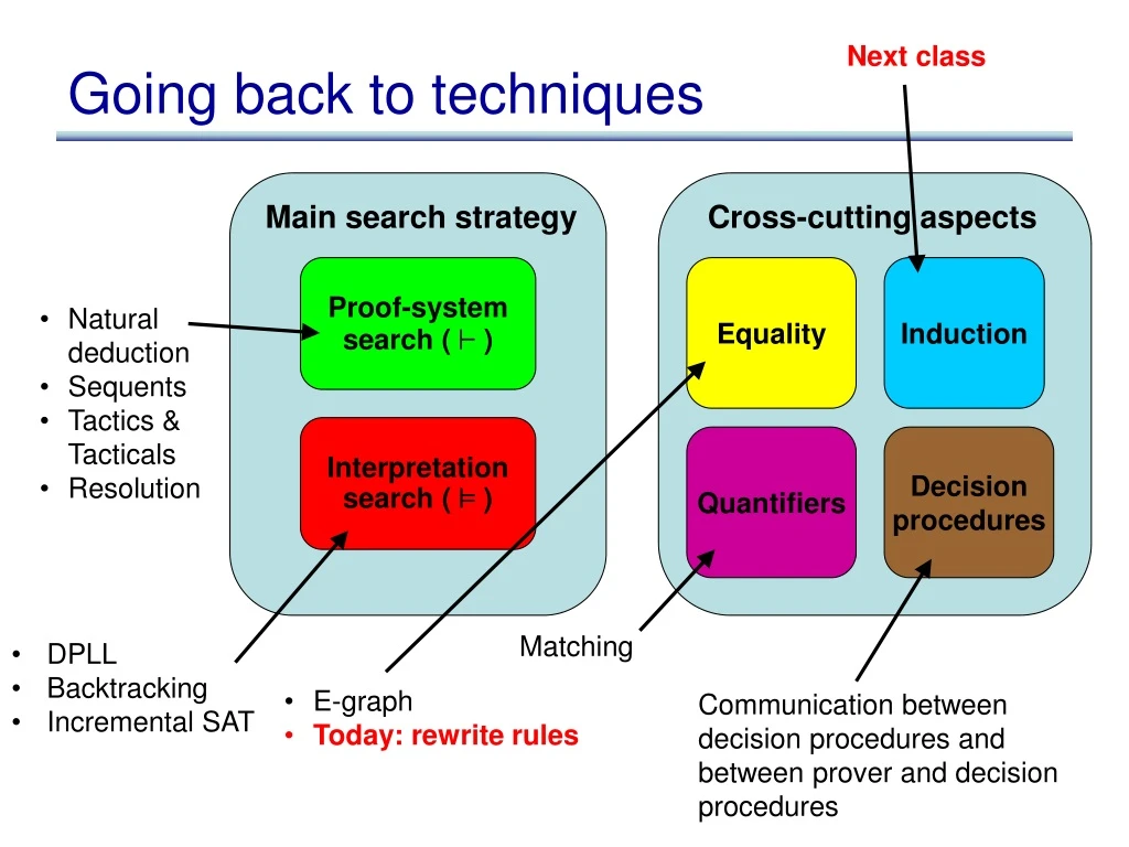
Main search strategy Cross-cutting aspects Proof-system search ( ` ) Equality Induction Interpretation search (² ) Quantifiers Decision procedures Next class Going back to techniques • Natural deduction • Sequents • Tactics & Tacticals • Resolution Matching • DPLL • Backtracking • Incremental SAT • E-graph • Today: rewrite rules Communication between decision procedures and between prover and decision procedures
Equality • We’ve seen one way of dealing with equality in this class: the E-graph • Another way to deal with equalities is to treat them as rewrite rules • An equality a = b can be used either as the rewrite rule a ! b or b ! a
Plan • First, we’ll see how rewrite rules are used in a few system • We’ll see some of the issues that come up • Then we’ll dig into the details • Formal foundations: rewrite systems • This is a huge area of work and research • We’ll see the snowflake on the tip of the iceberg
Rewrite rules in resolution • Show that the following is unsat: • { P(1), : P(f(0)), f(0) = 1 }
Rewrite rules in resolution • Show that the following is unsat: • { P(1), : P(f(0)), f(0) = 1 } • This technique is called demodulation
Resolution: another example • Show that the following is unsat: • { P(0), : P(f(0)), f(0) = 0 }
Resolution: another example • Show that the following is unsat: • { P(0), : P(f(0)), f(0) = 0 } • Which direction to pick • In the first example, can choose f(1) ! 1 or 1 ! f(1) • In the second example, pick f(0) ! 0 • Termination issues are cropping up
Rewrite rules in ACL2 • Recall ACL2 architecture: • Given a goal formula, try to apply various techniques in turn. Each technique generates sub-goals. Recurse on sub-goals. • Techniques: • Simplification • Instantiating known theorems • Term rewriting • As a last resort, induction
Rewrite rules in ACL2 • Rewrite rules in ACL2 are guarded • A rewrite rule is a lemma of the form: • h1Æ … Æ hn ) a = b • Here again, must pick a direction for the equality • Try to rewrite more “complicated” terms to “simpler” terms
Rewrite rules in ACL2 • ACL2 also uses local equality assumptions for performing rewrites • If lhs = rhs appears as a hypothesis in the goal, then replace lhs with rhs in rest of goal • Boyer and Moore call this cross-fertilization • More local than having rewrite lemmas
Performance issues • Heuristics for termination • Decreasing measure (guarantees termination “statically”) • Detect infinite loops and stop (can detect loops in the terms, or loops in the application of rules) • Or just have a timeout • One can also cache the results of rewriting • Rewriting can be expensive
Moving to the formal details… • We’ve seen some intuition for where to use rewrite rules • Now, let’s see some of the details • Rewrite rules have been studied in the context of term rewrite systems, which to are just sets of rewrite rules
Term rewrite systems • A term rewrite system is a pair (T, R) , where T is a set of terms and R is a set of rewrite rules of the form l1! l2 • T should actually be an algebra signature, but for our purposes, thinking of T as a set of terms is good enough • Rewrite rules can have free variables, but variables on the rhs must be a subset of variables on the lhs
Example 0 + y ! y s(x) + y ! s(x + y) fib(0) ! 0 fib(s(0)) ! s(0) fib(s(s(x))) ! fib(s(x)) + fib(x) • Run on: fib(s(s(s(0)))
Example 0 + y ! y s(x) + y ! s(x + y) fib(0) ! 0 fib(s(0)) ! s(0) fib(s(s(x))) ! fib(s(x)) + fib(x) • Run on: fib(s(s(s(0)))
A single rewrite step • We write t1! t2 to mean that term t1 rewrites to term t2 • s(0 + s(0)) ! s(s(0)) • Notice that the rewrite rule can be implied to a sub-term! • We need a way to formalize this
Contexts • A context C[¢] is a term with a “hole” in it: • C[¢] = s(0 + ¢) • The whole can be filled: • C[s(0)] = s(0 + s(0)) • When we write t1 = C[t2] , it means that term t2 appears inside t1, and C is the context inside which t2 appears
A single rewrite step • t1! t2 iff there exists a context C, and a rewrite rule l1! l2 such that:
A single rewrite step • t1! t2 iff there exists a context C, and a rewrite rule l1! l2 such that: • t1 = C[l1] • t2 = C[l2] • Can we show: • s(0 + s(0)) ! s(s(0)) • from rewrite rule s(x) + y ! s(x + y)
A single rewrite step • t1! t2 iff there exists a context C, a term t, a substitution , and a rewrite rule l1! l2 such that:
A single rewrite step • t1! t2 iff there exists a context C, a term t, a substitution , and a rewrite rule l1! l2 such that: • t1 = C[t] • = unify(l1, t) • t2 = C[( l2)]
Transitive closure of rewrites • !* is the reflexive transitive closure of ! • Another way to say the same: we write t1!* t2 to mean that there exists a possibly empty sequence s0 … sn such that: • t1! s0! … ! sn! t2
Termination • An term t is normal form or is irreducible if there is no term t’ such that t ! t’ • A rewrite system (T, R) is normalizing (also called weakly normalizing) if every t 2 T has a normal form • A rewrite system (T,R) is terminating (also called strongly normalizing) if there is no term t 2 T that will rewrite forever • What is the difference between strong and weak normalization?
Termination • One technique for showing termination: assign a measure to each term, and show that rewrite rules strictly decrease the measure • Example: s(p(x)) ! x p(s(x)) ! x minus(0) ! 0 minus(s(x)) ! p(minus(x))
Termination • Termination guarantees normalization • However, it does not guarantee that there is a unique normal form for a given term • We would like to have this additional uniqueness property • Confluence is the additional property we need
Confluence • Local confluence: for all terms a,b and c, if a ! b and a ! c, then there exists a term d such that b!* d and c !* d a b c d * *
Confluence • Local confluence: for all terms a,b and c, if a ! b and a ! c, then there exists a term d such that b!* d and c !* d a b c d * * a • Global confluence: for all terms a,b and c, if a ! * b and a !* c, then there exists a term d such that b!* d and c !* d * * b c d * *
Confluence • Local confluence: for all terms a,b and c, if a ! b and a ! c, then there exists a term d such that b!* d and c !* d a b c d * * when there exists a d such that b !* d and c !* d, we say that b and c are joinable a • Global confluence: for all terms a,b and c, if a ! * b and a !* c, then there exists a term d such that b!* d and c !* d * * b c d * *
Relation between local and global • Theorem: for a terminating system, local confluence implies global confluence • Proof by picture…
Canonical systems • A terminating and confluent system is canonical, meaning that each term has a unique canonical form • Simple decision procedure for such systems • To determine t1 = t2:
Canonical systems • A terminating and confluent system is canonical, meaning that each term has a unique canonical form • Simple decision procedure for such systems: • To determine t1 = t2:
Determining confluence • We would like an algorithm for determining whether a terminating system is confluent • To do this, we need to define the notion of critical pair
Critical pairs • Let l1! r1 and l2! r2 be rewrite rules that have no variables in common (rename vars if needed) • Suppose l1 = C[t] such that t is a non-trivial term (not a variable), and such that = unify(t,l2) • Then ((C[r2]),(r1)) is a critical pair • The intuition is that a critical pair represents a choice point: given a term l1=C[l2], we can either apply l1! r1 to get r1, or we can apply l2! r2 to get C[r2]
Critical pairs: example b(w(x)) ! w(w(w(b(x)))) w(b(y)) ! b(y) b(b(z)) ! w(w(w(w(z))))
Critical pairs: example b(w(x)) ! w(w(w(b(x)))) w(b(y)) ! b(y) b(b(z)) ! w(w(w(w(z))))
Critical pairs: another example s(p(x)) ! x p(s(x)) ! x minus(0) ! 0 minus(s(x)) ! p(minus(x))
Critical pairs: another example s(p(x)) ! x p(s(x)) ! x minus(0) ! 0 minus(s(x)) ! p(minus(x))
Critical pairs • Theorem: A term rewrite system is locally confluent if and only if all its critical pairs are joinable • Recall the meaning of joinable: b and c are joinable if there exists a d such that b !* d and c !* d • Corollary: A terminating rewrite system is confluent if and only if all its critical pairs are joinable
Algorithm for deciding confluence • Given a terminating rewrite system, find all critical pairs, and call this set CR
Algorithm for deciding confluence • Given a terminating rewrite system, find all critical pairs, and call this set CR • For each pair (s,t) 2 CR: • Find all the normal forms of s and t • Note: s and t are guaranteed to have normal forms because the system is terminating.
Algorithm for deciding confluence • Given a terminating rewrite system, find all critical pairs, and call this set CR • For each pair (s,t) 2 CR: • Find all the normal forms of s and t
Algorithm for deciding confluence • Given a terminating rewrite system, find all critical pairs, and call this set CR • For each pair (s,t) 2 CR: • Find all the normal forms of s and t • Let NS be the set of normal forms of s and NT be the set of normal forms of t
Algorithm for deciding confluence • Given a terminating rewrite system, find all critical pairs, and call this set CR • For each pair (s,t) 2 CR: • Find all the normal forms of s and t • Let NS be the set of normal forms of s and NT be the set of normal forms of t • If sizeof(NS) > 1 or sizeof(NT) > 1 return “NOT CONFLUENT” • (more than one normal form implies NOT confluent since confluence would imply unique normal form)
Algorithm for deciding confluence • Given a terminating rewrite system, find all critical pairs, and call this set CR • For each pair (s,t) 2 CR: • Find all the normal forms of s and t • Let NS be the set of normal forms of s and NT be the set of normal forms of t • If sizeof(NS) > 1 or sizeof(NT) > 1 return “NOT CONFLUENT” • If NS and NT are disjoint, return “NOT CONFLUENT” • Return “CONFLUENT”
What if the system is not confluent? • If we find a critical pair such that the normal forms are disjoint, add additional rewrite rules • This is called the Knuth-Bendix completion procedure
Knuth-Bendix completion procedure • Given a terminating rewrite system, find all critical pairs, and call this set CR • While there exists a critical pair (s,t) 2 CR such that the normal forms NS of s and the normals forms NT of t are disjoint: • For each s’ in NS, and for each term t’ in NT, add the rewrite rule s’ ! t’