Introduction to Haptic Rendering
Introduction to Haptic Rendering. Ming C. Lin lin@cs.unc.edu http://gamma.cs.unc.edu/interactive. What Is Haptic Rendering?. Master-Slave Systems. Human-in-the-Loop. Robot. Force Feedback. Haptic Device. Human. Simulation. Tactile Feedback. Virtual Reality.

Introduction to Haptic Rendering
E N D
Presentation Transcript
Introduction to Haptic Rendering Ming C. Lin lin@cs.unc.edu http://gamma.cs.unc.edu/interactive
What Is Haptic Rendering? Master-Slave Systems Human-in-the-Loop Robot Force Feedback Haptic Device Human Simulation Tactile Feedback Virtual Reality Pictures: http://haptic.mech.nwu.edu/intro/gallery/ M. C. Lin
Why Haptics? • Natural 3D interaction with a simulated environment. Not constrained by a 2D projection. • Additional sensorial input. Visual is dominant. Exploit extra dimensions, ‘cheat the user through the eyes’… In case of inconsistencies, visual wins. M. C. Lin
Inter-disciplinary Research Computer Science Electrical Engineering Mechanical Engineering Haptic Rendering Control and actuators Mechanical design Computation of the forces output by the device M. C. Lin
To be covered Haptic rendering for pen-type devices: Point-Object interaction Object-Object interaction • 3DOF Haptics(3D force output) • 6DOF Haptics (3D force + torque output) DOF = Degree of Freedom M. C. Lin
Some History • Argonne ’54, first master-slave systems. Master=slave. • Salisbury ’80, independent master and slave. Cartesian control of robot arm. Later, interaction with computer simulated slave (VR). • GROPE project UNC ’67-’90, molecular docking. • Minsky ’90, the Sandpaper. • Massie & Salisbury ’94, the Phantom. • Early 90’s to ’97, 3DOF haptics. • Late 90’s to today, 6DOF haptics. M. C. Lin
Control of Haptic Devices • Admittance devices • Impedance devices User x, v Simulation User F Simulation F Actuators F* x Actuators x* • Collision detection + contact response model • More popular • Collision detection + position constraints • Bulkier and more expensive • Very good for virtual walls M. C. Lin
6-DOF Phantom COBOTs Control of Haptic Devices • Admittance devices • Impedance Devices M. C. Lin
1KHz Performance Requirement • The user becomes part of the simulation loop. • 1KHz is necessary so that the whole system doesn’t suffer from disturbing oscillations. Think of the analogy with numerical integration of a system with spring, mass and damper, where the frequency of the haptic loop sets the integration step. • The Phantom haptic devices run their control loop at 1KHz. • Consequence: we are very limited on the amount of computation that we can do. M. C. Lin
Point-object Object-object 3DOF Haptics: Intro • Output: 3D force 3DOF haptics • Limited to applications where point-object interaction is enough. • Haptic visualization of data • Painting and sculpting • Some medical applications M. C. Lin
3DOF Haptics: Basic approach • Check if point penetrates an object. • Find closest point on the surface. • Penalty-based force. x F M. C. Lin
3DOF Haptics: The problems • Force discontinuities when crossing boundaries of internal Voronoi cells. Unexpected force discontinuities (both in magnitude and direction) are very disturbing! F2 F1 M. C. Lin
3DOF Haptics: The problems • Pop-through thin objects. After the mid line is crossed, the force helps popping through. motion M. C. Lin
3DOF Haptics: Point-to-plane • Mark et al., 1996. • For distributed applications. The simulator sends the equation of a plane to the haptic loop. The update of the plane is asynchronous. • Forces are computed between the haptic point and the plane. • Possible stiffness is limited, because too stiff would bring a jerky behavior at low update rates. M. C. Lin
3DOF Haptics: God-object • Zilles and Salisbury, 1995. • Use the position of the haptic interface point (HIP) and a set of local constraint surfaces to compute the position of god-object (GO). • Constraint surfaces defined using heuristics. • Compute GO as the point that minimizes the distance from HIP to the constraint surfaces. Lagrange multipliers. M. C. Lin
edge/vertex Concavity: 2/3 constraint planes in 3D motion motion 3DOF Haptics: God-object • Constraint surfaces: • Surfaces impeding motion • GO is outside (orientation test) and in the extension of the surface. • The HIP is inside the surface. M. C. Lin
3DOF Haptics: God-object • Constraint plane equations: • Energy function that will account for the distance. • Define cost function using Lagrange multipliers. • Minimize, solving for x, y, z, l1, l2 and l3. 3 planes at most M. C. Lin
3DOF Haptics: God-object • Partial derivatives on x, y, z, l1, l2 and l3 yield 6 linear equations: • In case of less than 3 planes, the problem has a lower dimension. M. C. Lin
3DOF Haptics: Virtual proxy • Ruspini et al., 1997. • Based on god-object. • Virtual proxy is a small sphere, instead of a point. Use configuration-space obstacles (C-obstacles), from robotics. • More formal definition of constraint planes. • Implementation of additional features, based on relocation of the virtual proxy. M. C. Lin
3DOF Haptics: Virtual proxy • C-obstacles: for a spherical object, is reduced to computing offset surfaces at a distance equal to the radius of the sphere. • Check the HIP against the offset surface. • This is done to avoid problems with small gaps in the mesh. M. C. Lin
3DOF Haptics: Virtual proxy • Finding the virtual proxy is based on an iterative search. • Basically, find subgoals based on the same distance minimization as for the god-object. • At each subgoal, all the planes that go through that point are potential constraints. The minimum set of active constraints is selected. • If the subgoal is in free space, set as new subgoal the HIP. The path might intersect the C-obstacles. Add the first plane intersected as a constraint and the intersection point as the current subgoal. • The process ends when the virtual proxy becomes stable. M. C. Lin
3DOF Haptics: Virtual proxy HIP(t) Perform collision detection between the path of the HIP and the C-obstacles HIP(t+Dt) M. C. Lin
3DOF Haptics: Virtual proxy HIP(t) Set the subgoal and the constraint plane(s) HIP(t+Dt) M. C. Lin
3DOF Haptics: Virtual proxy HIP(t) Find a new subgoal using the active planes and the minimization based on Lagrange multipliers HIP(t+Dt) M. C. Lin
3DOF Haptics: Virtual proxy HIP(t) Since the subgoal is in free space, drop the constraints, set the HIP as the new subgoal and perform collision detection between the path and the C-obstacles HIP(t+Dt) M. C. Lin
3DOF Haptics: Virtual proxy HIP(t) Recompute subgoal with new constraints HIP(t+Dt) M. C. Lin
3DOF Haptics: Virtual proxy HIP(t) The path to the new subgoal intersects another plane, so this is added to the set of constraints HIP(t+Dt) M. C. Lin
3DOF Haptics: Virtual proxy HIP(t) Compute active constraints (in 2D there are only 2) and find subgoal For this example, this is the final position of the virtual proxy HIP(t+Dt) M. C. Lin
3DOF Haptics: Virtual proxy • Quadratic programming approach: • The constraint planes define an open convex region (bounded by the plane at infinity). • The function to minimize is the distance from the haptic device (HIP) to the new subgoal (VPi+1): • The translation from the current location to the new subgoal cannot intersect the constraint planes. Define linear constraints based on the normals of the planes. Quadratic function Linear constraints M. C. Lin
Plane at Plane at Plane at Plane at Face (all surrounded by the plane at ) Edge Vertex 3DOF Haptics: Virtual proxy • Special case: simplified approach. • Let’s look at the convex region defined by the constraint planes M. C. Lin
3DOF Haptics: Virtual proxy • Normals (n) become points (-n) in a dual space (Gauss map). • The plane at infinity is the origin (o). • Points (-n) are joint together if the associated planes intersect. • The position of the virtual proxy also has a dual: • The vertices of the closest feature to P are the duals of the active constraint planes that are used for the minimization with Lagrange multipliers. M. C. Lin
3DOF Haptics: Virtual proxy M. C. Lin
3DOF Haptics: Virtual proxy • Force output: PD (proportional- derivative) control. Produces a force that will try to keep the VP and the HIP at the same position. VP F* F Simulation PD control Actuators HIP User It’s like a spring+damper, but the authors look at it from a control engineering approach M. C. Lin
v3 A1 A2 A3 v2 v1 3DOF Haptics: Additional features • Force shading by Basdogan et al., 1997. • Interpolate per-vertex normals using baricentric coordinates (same as Gouraud shading) • Effect: edges and vertices seem ‘rounded’ M. C. Lin
Force-shaded plane VP Original plane HIP’ HIP 3DOF Haptics: Additional features • Force shading by Ruspini et al., 1997. • Modify the position of the VP. • A subgoal (HIP’) is computed changing the normal of the plane. • This subgoal replaces the HIP, and the final VP is computed. M. C. Lin
3DOF Haptics: Additional features • Other effects by Ruspini et al., 1997. • Friction. • Textures. • Deformation. • All of them are achieved performing operations that modify the position of the VP. M. C. Lin
3DOF Haptics: Additional features • Friction by Hayward and Armstrong, 2000. • Model friction as an elasticity between the actual contact point (x) and a fictitious point, called adhesion point (w). • The adhesion point remains static or follows the actual contact depending on the ‘state’ (sliding, static…) w x M. C. Lin
3DOF Haptics: H-Collide • What about the collision detection? • Spatial uniform decomposition of space. Locate the path traversed by the probe in that grid, using a hash table. • Test the path against an OBBTree. Optimized test. • Use frame-to-frame coherence, caching the previous contact, and perform incremental computation. • When the leaf intersects, compute the surface contact point (SCP). Pass this to GHOST (haptic rendering library used by the Phantoms). M. C. Lin
3DOF Haptics: H-Collide Ray Vs. OBBTree test Spatial partitioning with hash table SCP computation SCP M. C. Lin
6DOF Haptics: Intro • Output: 3D force + 3D torque • For applications related to manipulation. • Assembly and maintenance oriented design. Removal of parts from complex structures. • Typical problem: peg-in-the-hole. There is a net torque M. C. Lin
6DOF Haptics: Intro • Formulate the problem as a rigid body simulation problem and output to the user the forces exerted on the object. Why not? • Too expensive • Constantly facing a situation of resting contacts. • Too much time performing collision detection to find non-penetrating situations. • Solve the linear complementarity problem. • Theoretically, it seems like the natural extension of the virtual proxy, though. M. C. Lin
Simulated object (xs, qs) com com com Haptic device (xh, qh) 6DOF Haptics: Intro The position of the center of mass (com) and the orientation cannot be governed directly by the haptic device. Interpenetrations would be unavoidable. M. C. Lin
Contact volume Contact area Contact points (e.g. local minima of distance function) 6DOF Haptics: Contacts • We cannot afford to compute ‘exact’ contacts. • Allow tolerances. Consider as valid contact whatever is inside a distance tolerance. • Outward offset surfaces are better. Distance is cheaper to compute than penetration. M. C. Lin
6DOF Haptics: Major approaches • All the approaches suffer from the fact that it’s an output-dependant problem. • Point cloud Vs. voxelized model. It can be linear on the number of points. The number of points grows quadratically with the resolution. • Polygonal models. At least linear on the number of convex pairs inside the tolerance. • NURBS. Very complex exact distance computation between NURBS surfaces. M. C. Lin
6DOF Haptics: Voxel sampling • McNeely et al., 1999. • Voxelize all the models in the scene. • For the haptic object, represent each voxel by a point Point Shell. • Test points against voxels of the scene. • Compute force at each point that penetrates an object. • Add up all the force and torque, and apply them to the user through virtual coupling. M. C. Lin
6DOF Haptics: Voxel sampling • All the objects are voxelized. • For the haptic object, store points at the center of the voxels, with inward normals determined by the polygonal model. • For the objects in the scene, create the voxmap, a 512-tree with 3 levels (the 512-tree is an extension of the octree, with 512 children per node, cube of 8*8*8). The 512-tree optimizes memory. • The initial implementation is only for static objects. M. C. Lin
6DOF Haptics: Voxel sampling Original object Voxels Pointshell M. C. Lin
interior surface proximity free space 6DOF Haptics: Voxel sampling • All the voxels in the voxmap store info about their position in the object: interior, surface, proximity or free space. M. C. Lin
6DOF Haptics: Voxel sampling • To start the collision query, all the pointshell has to be transformed to the local coordinates of the voxelized objects. • Points that are in the surface or proximity voxels are considered as contacts. M. C. Lin
N Take the plane with normal N that goes through the center of the voxel. Compute d as the distance from the point to that plane. d 6DOF Haptics: Voxel sampling • Forces at each contact are computed according to the tangent-plane force model. • Contacts are valid if d<0 (penetration). • If penetration to the interior happens, the contact is missed. One might think of computing a distance field in the interior, but the distance depends on the normal N. M. C. Lin