Understanding Arrival Patterns: Poisson Process & Exponential Distribution
Learn about arrival patterns, Poisson process, exponential distribution, merging streams, waiting for service, and more in queueing system components.

Understanding Arrival Patterns: Poisson Process & Exponential Distribution
E N D
Presentation Transcript
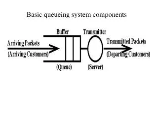
Arrivalpatterns • What is common to these arrival patterns? • What is different? • How can we describe/specify an arrival pattern?
Describing an arrival pattern 0 10 20 30 40 • N(t) = number of arrivals upto time t • {N(t), 0<t<40} is called a process • N(t) is a random variable for every timepoint t • To specify an arrival pattern, we must specify the probability distribution of N(t) for every time t
Describe an arrival process • E.g. N(t) = N(t,t) • What are reasonable t,t ? • Is this a reasonable process? • Let N(0) = 0, h a small interval of time • What is a reasonable distribution for N(h)? 0 10 20 30 40
The Poisson process • Small time interval h. Prob(event in interval h) = h • The probability of an event in h depends only on the length of h and not on its position, t. e.g, it does not matter how long since an event last occurred. The process has no memory. (sometimes called the Markovian property). • We choose to make h and small enough so that at most one event will occur in h. • is called the event rate or arrival rate
No events P(event in interval h) = h • P{0 events in interval [t, t+h] } = 1 - h (here h << 1) Define p0(t) = P{0 events in [0, t] } Then p0(t+h) = P{ 0 events in [0, t+h]} Since probability of an event in h is independent of any other: p0(t+h) = p0(t).(1 - h)
Poisson distribution P(N=k) = mke-m / k! Poisson process (rate = l) P(N(t)=k) = (lt)k e-lt / k!
How long before the next arrival? • T= time of next arrival • P(T>t) = P(N(t)=0) = e-lt • fT (t) = e- t (exponential distribution) • the average time between events = 1/ .
Exponential distribution l E(x)=l
Prob{event in stream 1 is in h } = 1hProb{event in stream 2 is in h } = 2h Prob{some event is in h} = Prob{stream 1 event} + Prob{stream 2 event} = 1 h + 2h = (1 + 2)h Merged stream acts like a Poisson process with rate = 1 + 2
Partitioning two streams • Whenever an event (arrival) occurs we divert it into A or B stream according to fixed probabilities, pA and pB. Prob{A event in h} = prob{event in h} × Prob{choosing A stream} = hpA • The A stream acts like a Poisson stream with a rate of events = pA
Poisson arrivals Random arrivals • Given: arrival has occurred in [0,t] • Let X = time to arrival • Then X ~ U[0,t] • Interpretation: arrival has occurred at random in [0,t] 0 t X
How long do you have to wait for service? • Red job already in service. Blue job comes into the queue (length 1). How long will blue have to wait (how much is R) ? • Assume job lengths are Exponentially distributed with average length • Then E(R) = (renewal paradox) T R
Residual time distribution T t R additional time to complete a service is independent of how long it has already been in service P(R>r) =P(T>r+t |T>t) =P(T>r+t)/P(T>t) = e-(r+t) /e-t = = e-r = P (T > r) time up to next arrival is independent of when the previous arrival occurred
How long between arrivals ? • Since no memory the zero point can be an event. • Thus time between events is also exponential, . • f(t) = e- t • the average time between events = 1/ .