A Basic Queueing System
A Basic Queueing System. Herr Cutter’s Barber Shop. Herr Cutter is a German barber who runs a one-man barber shop. Herr Cutter opens his shop at 8:00 A.M. The table shows his queueing system in action over a typical morning. Arrivals.
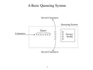

A Basic Queueing System
E N D
Presentation Transcript
Herr Cutter’s Barber Shop • Herr Cutter is a German barber who runs a one-man barber shop. • Herr Cutter opens his shop at 8:00 A.M. • The table shows his queueing system in action over a typical morning.
Arrivals • The time between consecutive arrivals to a queueing system are called the interarrival times. • The expected number of arrivals per unit time is referred to as the mean arrival rate. • The symbol used for the mean arrival rate is l = Mean arrival rate for customers coming to the queueing system where l is the Greek letter lambda. • The mean of the probability distribution of interarrival times is 1 / l = Mean interarrival time • Most queueing models assume that the form of the probability distribution of interarrival times is an exponential distribution.
Properties of the Exponential Distribution • There is a high likelihood of small interarrival times, but a small chance of a very large interarrival time. This is characteristic of interarrival times in practice. • For most queueing systems, the servers have no control over when customers will arrive. Customers generally arrive randomly. • Having random arrivals means that interarrival times are completely unpredictable, in the sense that the chance of an arrival in the next minute is always just the same. • The only probability distribution with this property of random arrivals is the exponential distribution. • The fact that the probability of an arrival in the next minute is completely uninfluenced by when the last arrival occurred is called the lack-of-memory property.
The Queue • The number of customers in the queue (or queue size) is the number of customers waiting for service to begin. • The number of customers in the system is the number in the queue plus the number currently being served. • The queue capacity is the maximum number of customers that can be held in the queue. • An infinite queue is one in which, for all practical purposes, an unlimited number of customers can be held there. • When the capacity is small enough that it needs to be taken into account, then the queue is called a finite queue. • The queue discipline refers to the order in which members of the queue are selected to begin service. • The most common is first-come, first-served (FCFS). • Other possibilities include random selection, some priority procedure, or even last-come, first-served.
Service • When a customer enters service, the elapsed time from the beginning to the end of the service is referred to as the service time. • Basic queueing models assume that the service time has a particular probability distribution. • The symbol used for the mean of the service time distribution is 1 / m = Mean service timewhere m is the Greek letter mu. • The interpretation of m itself is the mean service rate.m = Expected service completions per unit time for a single busy server
Some Service-Time Distributions • Exponential Distribution • The most popular choice. • Much easier to analyze than any other. • Although it provides a good fit for interarrival times, this is much less true for service times. • Provides a better fit when the service provided is random than if it involves a fixed set of tasks. • Standard deviation: s = Mean • Constant Service Times • A better fit for systems that involve a fixed set of tasks. • Standard deviation: s = 0. • Erlang Distribution • Fills the middle ground between the exponential distribution and constant. • Has a shape parameter, k that determines the standard deviation. • In particular, s = mean / (k)
Labels for Queueing Models To identify which probability distribution is being assumed for service times (and for interarrival times), a queueing model conventionally is labeled as follows: Distribution of service times — / — / — Number of Servers Distribution of interarrival times The symbols used for the possible distributions areM = Exponential distribution (Markovian)D = Degenerate distribution (constant times)Ek = Erlang distribution (shape parameter = k)GI = General independent interarrival-time distribution (any distribution)G = General service-time distribution (any arbitrary distribution)
Summary of Usual Model Assumptions • Interarrival times are independent and identically distributed according to a specified probability distribution. • All arriving customers enter the queueing system and remain there until service has been completed. • The queueing system has a single infinite queue, so that the queue will hold an unlimited number of customers (for all practical purposes). • The queue discipline is first-come, first-served. • The queueing system has a specified number of servers, where each server is capable of serving any of the customers. • Each customer is served individually by any one of the servers. • Service times are independent and identically distributed according to a specified probability distribution.
Examples of Commercial Service SystemsThat Are Queueing Systems
Examples of Internal Service SystemsThat Are Queueing Systems
Examples of Transportation Service SystemsThat Are Queueing Systems
Choosing a Measure of Performance • Managers who oversee queueing systems are mainly concerned with two measures of performance: • How many customers typically are waiting in the queueing system? • How long do these customers typically have to wait? • When customers are internal to the organization, the first measure tends to be more important. • Having such customers wait causes lost productivity. • Commercial service systems tend to place greater importance on the second measure. • Outside customers are typically more concerned with how long they have to wait than with how many customers are there.
Defining the Measures of Performance L = Expected number of customers in the system, including those being served (the symbol L comes from Line Length). Lq = Expected number of customers in the queue, which excludes customers being served. W = Expected waiting time in the system (including service time) for an individual customer (the symbol W comes from Waiting time). Wq = Expected waiting time in the queue (excludes service time) for an individual customer. These definitions assume that the queueing system is in a steady-state condition.
Relationship between L, W, Lq, and Wq • Little’s formula states thatL = lWandLq= lWq • Since 1/m is the expected service timeW = Wq+ 1/m • Combining the above relationships leads toL = Lq + l/m
Using Probabilities as Measures of Performance • In addition to knowing what happens on the average, we may also be interested in worst-case scenarios. • What will be the maximum number of customers in the system? (Exceeded no more than, say, 5% of the time.) • What will be the maximum waiting time of customers in the system? (Exceeded no more than, say, 5% of the time.) • Statistics that are helpful to answer these types of questions are available for some queueing systems: • Pn = Steady-state probability of having exactly n customers in the system. • P(W ≤ t) = Probability the time spent in the system will be no more than t. • P(Wq ≤ t) = Probability the wait time will be no more than t. • Examples of common goals: • No more than three customers 95% of the time: P0 + P1 + P2 + P3 ≥ 0.95 • No more than 5% of customers wait more than 2 hours: P(W ≤ 2 hours) ≥ 0.95
The Dupit Corp. Problem • The Dupit Corporation is a longtime leader in the office photocopier marketplace. • Dupit’s service division is responsible for providing support to the customers by promptly repairing the machines when needed. This is done by the company’s service technical representatives, or tech reps. • Current policy: Each tech rep’s territory is assigned enough machines so that the tech rep will be active repairing machines (or traveling to the site) 75% of the time. • A repair call averages 2 hours, so this corresponds to 3 repair calls per day. • Machines average 50 workdays between repairs, so assign 150 machines per rep. • Proposed New Service Standard: The average waiting time before a tech rep begins the trip to the customer site should not exceed two hours.
Alternative Approaches to the Problem • Approach Suggested by John Phixitt: Modify the current policy by decreasing the percentage of time that tech reps are expected to be repairing machines. • Approach Suggested by the Vice President for Engineering: Provide new equipment to tech reps that would reduce the time required for repairs. • Approach Suggested by the Chief Financial Officer: Replace the current one-person tech rep territories by larger territories served by multiple tech reps. • Approach Suggested by the Vice President for Marketing: Give owners of the new printer-copier priority for receiving repairs over the company’s other customers.
The Queueing System for Each Tech Rep • The customers: The machines needing repair. • Customer arrivals: The calls to the tech rep requesting repairs. • The queue: The machines waiting for repair to begin at their sites. • The server: The tech rep. • Service time: The total time the tech rep is tied up with a machine, either traveling to the machine site or repairing the machine. (Thus, a machine is viewed as leaving the queue and entering service when the tech rep begins the trip to the machine site.)
Notation for Single-Server Queueing Models • l = Mean arrival rate for customers = Expected number of arrivals per unit time1/l = expected interarrival time • m = Mean service rate (for a continuously busy server) = Expected number of service completions per unit time1/m = expected service time • r = the utilizationfactor= the average fraction of time that a server is busy serving customers = l / m
The M/M/1 Model • Assumptions • Interarrival times have an exponential distribution with a mean of 1/l. • Service times have an exponential distribution with a mean of 1/m. • The queueing system has one server. • The expected number of customers in the system is L = r / (1 –r) = l / (m– l) • The expected waiting time in the system is W = (1 / l)L = 1 / (m – l) • The expected waiting time in the queue is Wq= W – 1/m = l / [m(m – l)] • The expected number of customers in the queue is Lq= lWq = l2 / [m (m – l)]
The M/M/1 Model • Theprobability of having exactly n customers in the system is Pn = (1 – r)rnThus,P0 = 1 – rP1 = (1 – r)rP2 = (1 – r)r2 : : • The probability that the waiting time in the system exceeds t is P(W > t) = e–m (1–r)tfor t ≥ 0 • The probability that the waiting time in the queue exceeds t is P(Wq > t) = r e–m (1–r)tfor t ≥ 0
John Phixitt’s Approach (Reduce Machines/Rep) • The proposed new service standard is that the average waiting time before service begins be two hours (i.e., Wq≤ 1/4 day). • John Phixitt’s suggested approach is to lower the tech rep’s utilization factor sufficiently to meet the new service requirement. Lower r = l / m, until Wq≤ 1/4 day,wherel = (Number of machines assigned to tech rep) / 50.
M/M/1Model for John Phixitt’s Suggested Approach(Reduce Machines/Rep)
The M/G/1 Model • Assumptions • Interarrival times have an exponential distribution with a mean of 1/l. • Service times (T) can have any probability distribution. E(T) = 1/m , Var(T) = s2. 3. The queueing system has one server. • The probability of zero customers in the system is P0 = 1 – r • The expected number of customers in the queue is Lq= l2[Var(T)+ E(T)2] / [2(1 – lE(T))] • The expected number of customers in the system is L = Lq + l/m The expected waiting time in the queue is Wq= Lq/ l • The expected waiting time in the system is W = Wq+ 1/m
The Values of s and Lqfor the M/G/1 Modelwith Various Service-Time Distributions • The expected number of customers in the queue is Lq= l2[Var(T)+ E(T)2] / [2(1 – lE(T))]=[l2s2 + r2] / [2(1 – r)]
VP for Engineering Approach (New Equipment) • The proposed new service standard is that the average waiting time before service begins be two hours (i.e., Wq≤ 1/4 day). • The Vice President for Engineering has suggested providing tech reps with new state-of-the-art equipment that would reduce the time required for the longer repairs. • After gathering more information, they estimate the new equipment would have the following effect on the service-time distribution: • Decrease the mean from 1/4 day to 1/5 day. • Decrease the standard deviation from 1/4 day to 1/10 day.
M/G/1 Model for the VP of Engineering Approach(New Equipment)
The M/M/s Model • Assumptions • Interarrival times have an exponential distribution with a mean of 1/l. • Service times have an exponential distribution with a mean of 1/m. • Any number of servers (denoted by s). • With multiple servers, the formula for the utilization factor becomesr = l / smbut still represents that average fraction of time that individual servers are busy.
CFO Suggested Approach (Combine Into Teams) • The proposed new service standard is that the average waiting time before service begins be two hours (i.e., Wq≤ 1/4 day). • The Chief Financial Officer has suggested combining the current one-person tech rep territories into larger territories that would be served jointly by multiple tech reps. • A territory with two tech reps: • Number of machines = 300 (versus 150 before) • Mean arrival rate = l = 6 (versus l = 3 before) • Mean service rate = m = 4 (as before) • Number of servers = s = 2 (versus s = 1 before) • Utilization factor = r = l/sm = 0.75 (as before)
M/M/s Model for the CFO’s Suggested Approach(Combine Into Teams of Two)
CFO Suggested Approach (Teams of Three) • The Chief Financial Officer has suggested combining the current one-person tech rep territories into larger territories that would be served jointly by multiple tech reps. • A territory with three tech reps: • Number of machines = 450 (versus 150 before) • Mean arrival rate = l = 9 (versus l = 3 before) • Mean service rate = m = 4 (as before) • Number of servers = s = 3 (versus s = 1 before) • Utilization factor = r = l/sm = 0.75 (as before)
M/M/s Model for the CFO’s Suggested Approach(Combine Into Teams of Three)
The Four Approaches Under Considerations Decision: Adopt the third proposal
Some Insights About Designing Queueing Systems • When designing a single-server queueing system, beware that giving a relatively high utilization factor (workload) to the server provides surprisingly poor performance for the system. • Decreasing the variability of service times (without any change in the mean) improves the performance of a queueing system substantially. • Multiple-server queueing systems can perform satisfactorily with somewhat higher utilization factors than can single-server queueing systems. For example, pooling servers by combining separate single-server queueing systems into one multiple-server queueing system greatly improves the measures of performance. • Applying priorities when selecting customers to begin service can greatly improve the measures of performance for high-priority customers.
Economic Analysis of the Number of Servers to Provide • In many cases, the consequences of making customers wait can be expressed as a waiting cost. • The manager is interested in minimizing the total cost. TC = Expected total cost per unit time SC = Expected service cost per unit time WC = Expected waiting cost per unit timeThe objective is then to choose the number of servers so as to Minimize TC = SC + WC • When each server costs the same (Cs= cost of server per unit time), SC = Cs s • When the waiting cost is proportional to the amount of waiting (Cw = waiting cost per unit time for each customer), WC = Cw L
Acme Machine Shop • The Acme Machine Shop has a tool crib for storing tool required by shop mechanics. • Two clerks run the tool crib. • The estimates of the mean arrival rate l and the mean service rate (per server) m arel = 120 customers per hourm = 80 customers per hour • The total cost to the company of each tool crib clerk is $20/hour, so Cs= $20. • While mechanics are busy, their value to Acme is $48/hour, so Cw = $48. • Choose s so as to Minimize TC = $20s + $48L.