Download

1 / 35
400 likes | 847 Views
Tomography: Image Reconstruction from Projections. Ajit Rajwade , CS 663. Introduction.

E N D
Tomography: Image Reconstruction from Projections AjitRajwade, CS 663
Introduction The degree of absorption of X-Rays at each point is measured by an X-Ray absorption detector. This detector produces a 1D signal whose amplitude/intensity is directly proportional to the extent of absorption. Any point in the signal = sum of the absorptivity values across the path of a single ray in the X-Ray beam that spatially maps onto that point. The image is a simplification of a set of real biological tissues: example, an organ/tumor surrounded by a background consisting of soft, uniform tissue. The set of tissues is bombarded with an X-Ray beam. The tumor has higher rate of absorption as compared to the surrounding tissue. Source of image: Book by Gonzalez, 3rd edition
Introduction Given the 1D signal (called a projection signal), we try to reconstruct the original 2D image by smearing backwards along the direction of projection. This is called as back-projection. The 1D signal that was measured is duplicated along the columns of the image to be estimated (see the directions marked in yellow). Projection taken in a different direction (at 90 degrees to the original direction) Another back-projection Sum-total of the two back-projections Source of image: Book by Gonzalez, 3rd edition
Introduction • Given projections in K different directions, we can hope to reconstruct the original image by performing back-projection along all these directions, and adding up the results. • The shape of the object will be approximated better and better as K increases.
Even with many (32) back-projections, there is a blur artifact in the reconstruction. This is called as a “halo effect”. Source of image: Book by Gonzalez, 3rd edition
Reconstructing 3D objects • A 3D object is illuminated with a large cone-shaped X-Ray beam. This will produce a projection which is a 2D-image. • Changing the direction of the X-ray beam will produce another image. This set of images when back-projected will yield the 3D volume/object. • However in conventional Computed Tomography (CT), each slice of the volume is measured at a time. A slice is a 2D entity obtained by cutting the 3D volume transversely through a plane parallel to the XY plane. • This allows for the employment of a smaller number of detectors at a time, for the same resolution of the measurement.
Z X Y X-Ray Image I0
Parameterization of a direction/line The direction of projection is denoted L, and dL is an infinitesimally small element along L. L is parameterized as follows (the “normal representation of the line”): Source of image: Book by Gonzalez, 3rd edition
Source of image: Book by Gonzalez, 3rd edition Given a direction ϴ, the source and detector pair move along that direction in fixed steps (i.e. variation in ρ). The distance between source and detector is constant. At each step, the source sends out an X-Ray beam onto the subject, and the projection value is recorded on the detector and stored in a computer. This process is repeated for several values of ϴ. In the end, we record a single 2D slice. Now, the subject is moved in a direction perpendicular to the plane of the source-detector pair, and another 2D slice is recorded. This is called 1st generation CT.
Source of image: Book by Gonzalez, 3rd edition In second-generation CT, the source sends out an X-ray beam in the form of a cone (also called fan). There are more detectors needed, but fewer translations are required to record a single 2D slice (rotations are needed just as before). In third-generation CT, the source sends out an X-ray beam in the form of a large cone. The number of detectors is long enough to cover the field of view, so no translations are needed to record a single 2D slice (only rotations are needed).
In fourth-generation CT, there is a large number of detectors arranged in the form of a circle. The source alone rotates. Source of image: Book by Gonzalez, 3rd edition
Aim of Tomography • To estimate the full 3D structure of an object from its projections. • The projections are directly measured, the 3D structure is estimated. • Applications: medical imaging, industrial applications such as fault detection in machines, observation of plant roots, remotesensing (observation of underground objects or phenomena).
Representing Projections • The complete set of projections for several different values of the parameters ρ and ϴ gives: • This is called the Radon Transform of f. Its discrete version is: Dirac delta function One projection is obtained with a fixed value of ϴ, but varying ρ. Kronecker delta function
Example: Source of image: Book by Gonzalez, 3rd edition
-90 0 +90 Sinogram (a radon transform plotted as an image in a (ρ,ϴ) grid. Non-zero portion of the 90 degree row in the sinogram is smaller than the non-zero portion of the 0-degree row. This means the object width is smaller than its height. Sinogram is symmetric in both directions means that the original object is symmetric about X and Y axes, and parallel to the axes. -90 0 +90 Source of image: Book by Gonzalez, 3rd edition
Back-projection Radon transform: obtained by sampling several different angles Fix the angle ϴk and for all x and y, compute the value of ρ. Copy g(ρ, ϴk) to hat(f)ϴk(x,y), which is the image obtained when you back-project along angle ϴk. The back-projection operator is NOT the same as the inverse of the Radon transform! So this does not yield back the true signal f(x,y), but the signal f(x,y) blurred with the kernel (x2+y2)-0.5. More on this a few slides down, when we do filtered back-projection.
The blur is a painful consequence of (1) discretization of the angle ϴ, and (2) the inherent blurring with the kernel (x2+y2)-0.5. These images are reconstructed at 0.5 degree changes in ϴ. How do we get rid of this blur? Wait for a few slides! Source of image: Book by Gonzalez, 3rd edition
Fourier transform of the Radon Transform • The Radon transform is given as: • Its 1D Fourier transform w.r.t. ρ (keeping ϴ fixed to some value) is given by: G(μ, ϴ) is the Fourier transform of the projection of f(x,y) along some direction ϴ.
Fourier transform of the Radon Transform • Its 1D Fourier transform w.r.t. ρ (keeping ϴ fixed) is given by: The RHS of this equation is a slice of the 2D Fourier transform of f(x,y), i.e. F(u,v), along the angle ϴ in the frequency plane, and passing through the origin This equation above is called the Projection Slice Theorem or the Fourier Slice Theorem. It states that the Fourier transform of a projection of the 2D object along some direction ϴ (i.e. G(μ, ϴ)) is equal to a slice of the 2D Fourier transform of the object along the same direction ϴ (in the frequency plane), passing through the origin.
The Projection Slice Theorem or the Fourier Slice Theorem states that the following two are equivalent: Project a 2D object along a certain direction d. Take its 1D Fourier Transform called as F1. Compute the 2D Fourier transform of the same object. Take a slice of this Fourier transform along a direction parallel to d (but in the frequency plane). Call this slice as F2. Now F1 = F2. Source of image: Book by Gonzalez, 3rd edition
Filtered Back-projection • Consider the 2D inverse Fourier transform of F(u,v), giving us: • Consider u = μcos(Ѳ), v = μ sin(Ѳ). Then: Note: we are doing a change of variables from (u,v) to (μ,Ѳ). Hence du dv = μ dμ dѲ.
Filtered Back-projection • By projection slice theorem, this becomes: • Further simplification will give the following (see next slide)
Filtered Back-projection This is a 1D Inverse Fourier Transform with an added term |μ| (a ramp filter). But this function is not integrable as |μ| grows unboundedly. Hence the inverse Fourier transform does not exist! |μ| μ
Filtered Back-projection versus back-projection This is a 1D Inverse Fourier Transform with an added term |μ| (a ramp filter). But this function is not integrable as |μ| grows unboundedly. Hence the inverse Fourier transform does not exist! Now suppose that additional term |μ| were absent. We would then obtain simple back-projection:
Filtered Back-projection algorithm: version 1 • The X-Ray or CT machine gives you projections (i.e. Radon transforms) of the data in different directions. • Perform simple back-projection to get a 2D image. • Convolve it with the kernel (x2+y2)^0.5 to get the final image OR Find the 2D Fourier transform of the back-projected 2D image and multiply it with (u2+v2)^0.5 and find the 2D inverse Fourier Transform of the product.
Filtered Back-Projection • In practice, the ramp filter is multiplied in the frequency domain by a windowing function (equivalent to convolution with the corresponding kernel in the spatial domain). • It has the advantage of controlling some amount of noise. • The simplest windowing function is a rect. • This formula is called the RamachandranLakshminarayanan (Ram-Lak) filter. http://www.pnas.org/content/68/9/2236
Ram-Lak filter: ramp multiplied by rect (both in frequency domain) Other windowing functions can also be used! (eg: Hamming window, which is a truncated cosine). These windowing functions allow lesser ringing artifacts as compared to the rect windowing function. Source of image: Book by Gonzalez, 3rd edition
Ram-Lak filter Ram-Lak filter with Hamming window
Filtered Back-projection algorithm: version 2 (faster) • Compute the 1D Fourier transform of each projection of the object (the projections are measured by the X-Ray or CT machine). • Multiply each Fourier transform by the ramp filter |μ| multiplied by a windowing function (such as rect, or Hamming). • Obtain the 1D inverse Fourier transform of the result. • Sum up over all such results (one each per projection angle) from the previous step to give the final image.
Properties of the Radon Transform • Linearity: • Symmetry: • Shifting: • Scaling:
Properties of the Radon Transform • Convolution: The Radon transform of a 2D convolution of two functions is equal to the convolution of their Radon Transforms.
Properties of Radon Transform • The convolution property is very useful as it allows for replacement of a 2D convolution by a 1D convolution after computing the Radon transform.