Association Analysis: Concepts & Algorithms
330 likes | 360 Views
Understand frequent itemset generation, rule evaluation, and compact representation for efficient association rule mining. Learn about FP-Growth algorithm and evaluation of association patterns.

Association Analysis: Concepts & Algorithms
E N D
Presentation Transcript
UNIT 4-Association Analysis : Basic Concepts and Algorithms • Frequent Itemset Generation • Rule Generation • Compact Representation of Frequent Itemsets • Alternative methods for generating Frequent Itemsets • FP Growth Algorithm • Evaluation of Association Patterns
Itemset • A collection of one or more items • Example: {Milk, Bread, Diaper} • k-itemset • An itemset that contains k items • Support count () • Frequency of occurrence of an itemset • E.g. ({Milk, Bread,Diaper}) = 2 • Support • Fraction of transactions that contain an itemset • E.g. s({Milk, Bread, Diaper}) = 2/5 • Frequent Itemset • An itemset whose support is greater than or equal to a minsup threshold
Example: • Association Rule • An implication expression of the form X Y, where X and Y are itemsets • Example: {Milk, Diaper} {Beer} • Rule Evaluation Metrics • Support (s) • Fraction of transactions that contain both X and Y • Confidence (c) • Measures how often items in Y appear in transactions thatcontain X
Given a set of transactions T, the goal of association rule mining is to find all rules having • support ≥ minsup threshold • confidence ≥ minconf threshold • Brute-force approach: • List all possible association rules • Compute the support and confidence for each rule • Prune rules that fail the minsup and minconf thresholds • Computationally prohibitive! • Frequent Itemset Generation • Generate all itemsets whose support minsup
Generate high confidence rules from each frequent itemset, where each rule is a binary partitioning of a frequent itemset • Given a frequent itemset L, find all non-empty subsets f L such that f L – f satisfies the minimum confidence requirement • If {A,B,C,D} is a frequent itemset, candidate rules: • ABC D, ABD C, ACD B, BCD A, A BCD, B ACD, C ABD, D ABCAB CD, AC BD, AD BC, BC AD, BD AC, CD AB, • If |L| = k, then there are 2k – 2 candidate association rules (ignoring L and L)
How to efficiently generate rules from frequent itemsets? • In general, confidence does not have an anti-monotone property c(ABC D) can be larger or smaller than c(AB D) • But confidence of rules generated from the same itemset has an anti-monotone property • e.g., L = {A,B,C,D}: c(ABC D) c(AB CD) c(A BCD) • Confidence is anti-monotone w.r.t. number of items on the RHS of the rule
Pruned Rules Rule Generation for Apriori Algorithm Lattice of rules Low Confidence Rule
Candidate rule is generated by merging two rules that share the same prefixin the rule consequent • join(CD=>AB, BD=>AC)would produce the candidaterule D => ABC • Prune rule D => ABC if itssubset AD => BC does not havehigh confidence
Maximal Frequent Itemset An itemset is maximal frequent if none of its immediate supersets is frequent Maximal Itemsets Infrequent Itemsets Border
Closed Itemset • An itemset is closed if none of its immediate supersets has the same support as the itemset
Maximal vs Closed Itemsets Transaction Ids Not supported by any transactions
Traversal of Itemset Lattice • General-to-specific vs Specific-to-general
Traversal of Itemset Lattice • Equivalent Classes
Traversal of Itemset Lattice • Breadth-first vs Depth-first
Representation of Database • horizontal vs vertical data layout
FP-growth Algorithm • Use a compressed representation of the database using an FP-tree • Once an FP-tree has been constructed, it uses a recursive divide-and-conquer approach to mine the frequent itemsets
FP Tree Construction null After reading TID=1: A:1 B:1 After reading TID=2: null B:1 A:1 B:1 C:1 D:1
FP Tree Construction Transaction Database null B:3 A:7 B:5 C:3 C:1 D:1 Header table D:1 C:3 E:1 D:1 E:1 D:1 E:1 D:1 Pointers are used to assist frequent itemset generation
FP Growth Conditional Pattern base for D: P = {(A:1,B:1,C:1), (A:1,B:1), (A:1,C:1), (A:1), (B:1,C:1)} Recursively apply FP-growth on P Frequent Itemsets found (with sup > 1): AD, BD, CD, ACD, BCD null A:7 B:1 B:5 C:1 C:1 D:1 D:1 C:3 D:1 D:1 D:1
Subjective Interestingness • Visualization • Domain experts to interact with the data mining system by interpreting and verifying the discovered patterns • Template based approach • Instead of reporting all the extracted rules, only rules that satisfy a user specified template are returned. • Subjective interestingness measures • Defined based on domain information or profit margin of items. The measures can then be used to filter patterns that are obvious and non-actionable.
Objective Interestingness • Domain independent • Computed based on contingency table A 2-way contingency table for variables A and B
Limitations of the Support-Confidence Framework {Tea} {Coffee} Support = 15%, Confidence = 75% Coffee drinker = 80% Tea and Coffee drinker =75% A tea drinker actually decreases her probability of being a coffee drinker from 80% to 75%, Beverage preference hence, the rule {Tea} {Coffee}is misleading • Pitfalls: Confidence traced to the fact that the measure ignores the support of the itemset in the rule consequent.
Interest Factor • Lift or Interest Factor = i.e.
Measures beyond Pairs of Binary Variables 3-dimensional contingency table
Measures beyond Pairs of Binary Variables Buy Exercise Machine Yes No Buy Exercise Machine Yes No
Simpson’s Paradox • The rule {HDTV = Yes} {Exercise Machine = Yes} has a confidence of 99/180 = 55% and the rule {HDTV = No} {Exercise Machine = Yes} has confidence of 54/120 = 45%. • College Students • c({HDTV = Yes} {Exercise Machine = Yes}) = 1/10 = 10% • c({HDTV = No} {Exercise Machine = Yes}) = 4/34 = 11.8% • Working Adults • c({HDTV = Yes} {Exercise Machine = Yes}) = 98/170 = 57.7% • c({HDTV = No} {Exercise Machine = Yes}) = 50/86 = 58.1% i.e. customers who do NOT buy HDTV are more likely to buy exercise machines, which contradicts the previous conclusion.
Simpson’s Paradox • Most customers who buy HDTV’s are working adults. • Working adults are also the largest group of customers who buy exercise machines. • Because 85% of customers are working adults, the observed relationship between HDTV and exercise machine turns out to be stronger in the combined data than what it would have been if the data is stratified.