Partitioning Algorithms: Basic Concepts
Partitioning Algorithms: Basic Concepts. Partition n objects into k clusters Optimize the chosen partitioning criterion Example: minimize the Squared Error Squared Error of a cluster m i is the mean (centroid) of C i Squared Error of a clustering. Example of Square Error of Cluster.

Partitioning Algorithms: Basic Concepts
E N D
Presentation Transcript
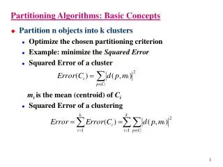
Partitioning Algorithms: Basic Concepts • Partition n objects into k clusters • Optimize the chosen partitioning criterion • Example: minimize the Squared Error • Squared Error of a cluster miis the mean (centroid) of Ci • Squared Error of a clustering
Example of Square Error of Cluster Ci={P1, P2, P3} P1 = (3, 7) P2 = (2, 3) P3 = (7, 5) mi = (4, 5) |d(P1, mi)|2 =(3-4)2+(7-5)2=5 |d(P2, mi)|2=8 |d(P3, mi)|2=9 Error (Ci)=5+8+9=22 10 9 8 7 6 5 4 3 2 1 P1 P3 P2 mi 0 1 2 3 4 5 6 7 8 9 10
Example of Square Error of Cluster Cj={P4, P5, P6} P4 = (4, 6) P5 = (5, 5) P6 = (3, 4) mj = (4, 5) |d(P4, mj)|2 =(4-4)2+(6-5)2=1 |d(P5, mj)|2=1 |d(P6, mj)|2=1 Error (Cj)=1+1+1=3 10 9 8 7 6 5 4 3 2 1 P4 P5 mj P6 0 1 2 3 4 5 6 7 8 9 10
Partitioning Algorithms: Basic Concepts • Global optimal: examine all possible partitions • kn possible partitions, too expensive! • Heuristic methods: k-means and k-medoids • k-means (MacQueen’67): Each cluster is represented by center of cluster • k-medoids (Kaufman & Rousseeuw’87): Each cluster is represented by one of the objects (medoid) in cluster
K-means • Initialization • Arbitrarily choose k objects as the initial cluster centers (centroids) • Iteration until no change • For each object Oi • Calculate the distances between Oi and the k centroids • (Re)assign Oi to the cluster whose centroid is the closest to Oi • Update the cluster centroids based on current assignment
cluster mean k-Means Clustering Method current clusters objects relocated new clusters
Example • For simplicity, 1 dimensional objects and k=2. • Objects: 1, 2, 5, 6,7 • K-means: • Randomly select 5 and 6 as initial centroids; • => Two clusters {1,2,5} and {6,7}; meanC1=8/3, meanC2=6.5 • => {1,2}, {5,6,7}; meanC1=1.5, meanC2=6 • => no change. • Aggregate dissimilarity = 0.5^2 + 0.5^2 + 1^2 + 1^2 = 2.5
Variations of k-Means Method • Aspects of variants of k-means • Selection of initial k centroids • E.g., choose k farthest points • Dissimilarity calculations • E.g., use Manhattan distance • Strategies to calculate cluster means • E.g., update the means incrementally
Strengths of k-Means Method • Strength • Relatively efficient for large datasets • O(tkn) where n is # objects, k is # clusters, and t is # iterations; normally, k, t <<n • Often terminates at a local optimum • global optimum may be found using techniques such as deterministic annealing and genetic algorithms
Weakness of k-Means Method • Weakness • Applicable only when mean is defined, then what about categorical data? • k-modes algorithm • Unable to handle noisy data and outliers • k-medoids algorithm • Need to specify k, number of clusters, in advance • Hierarchical algorithms • Density-based algorithms
k-modes Algorithm • Handling categorical data: k-modes (Huang’98) • Replacing means of clusters with modes • Given n records in cluster, mode is record made up of most frequent attribute values • In the example cluster, mode = (<=30, medium, yes, fair) • Using new dissimilarity measures to deal with categorical objects
+ + A Problem of K-means • Sensitive to outliers • Outlier: objects with extremely large (or small) values • May substantially distort the distribution of the data Outlier
10 9 8 7 6 5 4 3 2 1 0 0 1 2 3 4 5 6 7 8 9 10 k-Medoids Clustering Method • k-medoids: Find krepresentative objects, called medoids • PAM (Partitioning Around Medoids, 1987) • CLARA (Kaufmann & Rousseeuw, 1990) • CLARANS (Ng & Han, 1994): Randomized sampling k-means k-medoids
PAM (Partitioning Around Medoids) (1987) • PAM (Kaufman and Rousseeuw, 1987) • Arbitrarily choose k objects as the initial medoids • Until no change, do • (Re)assign each object to the cluster with the nearest medoid • Improve the quality of the k-medoids (Randomly select a nonmedoid object, Orandom, compute the total cost of swapping a medoid with Orandom) • Work for small data sets (100 objects in 5 clusters) • Not efficient for medium and large data sets
Swapping Cost • For each pair of a medoid m and a non-medoid object h, measure whether h is better than m as a medoid • Use the squared-error criterion • Compute Eh-Em • Negative: swapping brings benefit • Choose the minimum swapping cost
Four Swapping Cases • When a medoid m is to be swapped with a non-medoid object h, check each of other non-medoid objects j • j is in cluster of m reassign j • Case 1: j is closer to some k than to h; after swapping m and h, j relocates to cluster represented by k • Case 2: j is closer to h than to k; after swapping m and h, j is in cluster represented by h • j is in cluster of some k, not mcompare k with h • Case 3: j is closer to some k than to h; after swapping m and h, j remains in cluster represented by k • Case 4: j is closer to h than to k; after swapping m and h, j is in cluster represented by h
PAM Clustering: Total swapping cost TCmh=jCjmh - C = d ( j, h ) d ( j, k ) < 0 jmh Case 1 Case 3 j k h j h m k m Case 2 Case 4 k h j m m h j k
Complexity of PAM • Arbitrarily choose k objects as the initial medoids • Until no change, do • (Re)assign each object to the cluster with the nearest medoid • Improve the quality of the k-medoids • For each pair of medoid m and non-medoid object h • Calculate the swapping cost TCmh =jCjmh O(1) O((n-k)2*k) O((n-k)*k) O((n-k)2*k) (n-k)*k times O(n-k)
Strength and Weakness of PAM • PAM is more robust than k-means in the presence of outliers because a medoid is less influenced by outliers or other extreme values than a mean • PAM works efficiently for small data sets but does not scale well for large data sets • O(k(n-k)2 ) for each iteration where n is # of data objects, k is # of clusters • Can we find the medoids faster?
CLARA (Clustering Large Applications) (1990) • CLARA (Kaufmann and Rousseeuw in 1990) • Built in statistical analysis packages, such as S+ • It draws multiple samples of data set, applies PAM on each sample, gives best clustering as output • Handle larger data sets than PAM (1,000 objects in 10 clusters) • Efficiency and effectiveness depends on the sampling
CLARA - Algorithm • Set mincost to MAXIMUM; • Repeat q times // draws q samples • Create S by drawing s objects randomly from D; • Generate the set of medoids M from S by applying the PAM algorithm; • Compute cost(M,D) • If cost(M, D)<mincost Mincost = cost(M, D); Bestset = M; • Endif; • Endrepeat; • Return Bestset;
Complexity of CLARA • Set mincost to MAXIMUM; • Repeat q times • Create S by drawing s objects randomly from D; • Generate the set of medoids M from S by applying the PAM algorithm; • Compute cost(M,D) • If cost(M, D)<mincost Mincost = cost(M, D); Bestset = M; Endif; • Endrepeat; • Return Bestset; O(1) O((s-k)2*k+(n-k)*k) O(1) O((s-k)2*k) O((n-k)*k) O(1)
Strengths and Weaknesses of CLARA • Strength: • Handle larger data sets than PAM (1,000 objects in 10 clusters) • Weakness: • Efficiency depends on sample size • A good clustering based on samples will not necessarily represent a good clustering of whole data set if sample is biased
CLARANS (“Randomized” CLARA) (1994) • CLARANS (A Clustering Algorithm based on Randomized Search) (Ng and Han’94) • CLARANS draws sample in solution space dynamically • A solution is a set of k medoids • The solutions space contains solutions in total • The solution space can be represented by a graph where every node is a potential solution, i.e., a set of k medoids
Graph Abstraction • Every node is a potential solution (k-medoid) • Every node is associated with a squared error • Two nodes are adjacent if they differ by one medoid • Every node has k(nk) adjacent nodes {O1,O2,…,Ok} k(nk) neighbors for one node … … {Ok+1,O2,…,Ok} {Ok+n,O2,…,Ok} n-kneighbors for one medoid
Graph Abstraction: CLARANS • Start with a randomly selected node, check at most m neighbors randomly • If a better adjacent node is found, moves to node and continue; otherwise, current node is local optimum; re-starts with another randomly selected node to search for another local optimum • When h local optimum have been found, returns best result as overall result
N C N … … … … N N Local minimum Local minimum Local minimum Local minimum C numlocal N N CLARANS Compare no more than maxneighbortimes < Best Node
CLARANS - Algorithm • Set mincost to MAXIMUM; • For i=1 to h do // find h local optimum • Randomly select a node as the current node C in the graph; • J = 1; // counter of neighbors • Repeat Randomly select a neighbor N of C; If Cost(N,D)<Cost(C,D) Assign N as the current node C; J = 1; Else J++; Endif; • Until J > m • Update mincost with Cost(C,D) if applicableEnd for; • End For • Return bestnode;
Graph Abstraction (k-means, k-modes, k-medoids) • Each vertex is a set of k-representative objects (means, modes, medoids) • Each iteration produces a new set of k-representative objects with lower overall dissimilarity • Iterations correspond to a hill descent process in a landscape (graph) of vertices
Comparison with PAM • Search for minimum in graph (landscape) • At each step, all adjacent vertices are examined; the one with deepest descent is chosen as next k-medoids • Search continues until minimum is reached • For large n and k values (n=1,000, k=10), examining all k(nk) adjacent vertices is time consuming; inefficient for large data sets • CLARANS vs PAM • For large and medium data sets, it is obvious that CLARANS is much more efficient than PAM • For small data sets, CLARANS outperforms PAM significantly
When n=80, CLARANS is 5 times faster than PAM, while the cluster quality is the same.
Comparision with CLARA • CLARANS vs CLARA • CLARANS is always able to find clusterings of better quality than those found by CLARA; CLARANS may use much more time than CLARA • When the time used is the same, CLARANS is still better than CLARA
Hierarchies of Co-expressed Genes and Coherent Patterns The interpretation of co-expressed genes and coherent patterns mainly depends on the domain knowledge
group A1 group A A Subtle Situation • To split or not to split? It’s a question. group A2