Devising a scoring system
E N D
Presentation Transcript
DNA Properties and Genetic Sequence AlignmentCSE, Marmara University mimoza.marmara.edu.tr/~m.sakalli/cse546Nov/8/09
Devising a scoring system • Importance: • Scoring matrices appear in all analysis involving sequence comparison. • The choice of matrix can strongly influence the outcome of the analysis. • Understanding theories underlying a given scoring matrix can aid in making proper choice: • Some matrices reflect similarity: good for database searching • Some reflect distance: good for phylogenies • Log-odds matrices,a normalisation method for matrix values: • S is the probability that two residues, i and j, are aligned by evolutionary descent and by chance. • qij are the frequencies that i and j are observed to align in sequences known to be related. pi and pj are their frequencies of occurrence in the set of sequences.
A T C G T A C w 1 2 3 4 5 6 7 0 v 0 A 1 T 2 G 3 T 4 T 5 A 6 T 7 www.bioalgorithms.info\Winfried Just Next week: Aligning Two Strings Represents each row and each column with a number and a symbol of the sequence present up to a given position. For example the sequences are represented as: Alignment as a Path in the Edit Graph 0 1 2 2 3 4 5 6 7 7 A T _ G T T A T _ A T C G T _ A _ C 0 1 2 3 4 5 5 6 6 7 (0,0) , (1,1) , (2,2), (2,3), (3,4), (4,5), (5,5), (6,6), (7,6), (7,7)
A T C G T A C w 1 2 3 4 5 6 7 0 v 0 A 1 T 2 G 3 T 4 T 5 A 6 T 7 and represent indels (insertions and deletions) in v and wscoring 0. represent exact matches scoring 1. The score of the alignment path in the graph is 5. Every path in the edit graph corresponds to an alignment: Alternative Alignment 0122345677 v= AT_GTTAT_ w= ATCGT_A_C 0123455667 v= AT_GTTAT_ w= ATCG_TA_C
A T C G T A C w 1 2 3 4 5 6 7 0 0 0 0 0 0 0 0 0 0 v A 1 1 1 1 1 1 1 1 T 1 2 0 G 1 3 0 T 1 4 0 T 1 5 0 A 1 6 0 1 T 7 0 0 Alignment: Dynamic Programming ??? Use this scoring algorithm Si-1, j-1+1 if vi = wj Si,j =MAXSi-1, j value from top Si, j-1 value from left There are no matches at the beginning of the alignment First column row i=1, and row j=1 all labeled to be all zero {
A A T T C C G G T T A A C C w w v v A A T T 0 0 G G 0 0 0 0 0 0 0 0 0 0 1 1 1 1 1 T T 0 0 1 2 2 2 2 T T 0 0 1 2 2 3 3 3 A A 1 0 0 2 3 4 4 1 2 T T 3 4 4 0 0 2 2 3 4 5 0 0 1 2 3 5 5 Backtracking Example 1 2 3 4 5 6 7 0 Find a match in row and column 2. i=2, j=2,5 is a match (T). j=2, i=4,5,7 is a match (T). Since vi = wj, S(i,j) = Si-1,j-1 +1 S(2,2) = [S(1,1) = 1] + 1 S(2,5) = [S(1,4) = 1] + 1 S(4,2) = [S(3,1) = 1] + 1 S(5,2) = [S(4,1) = 1] + 1 S(7,2) = [S(6,1) = 1] + 1 The simplest form of a sequence similarity analysis, and solution to Longest Common Subsequence (LCS) problem 0 0 0 0 0 0 0 0 0 1 1 1 1 1 1 1 1 2 1 2 2 2 2 2 2 3 1 2 4 1 2 5 1 2 6 1 2 1 7 2 1 2 3 4 5 6 7 0 0 1 1 1 2 2 2 3 3 2 4 4 0122345677 0122345677 v= AT_GTTAT_ AT_GTTAT_ w= ATCGT_A_C ATCG_TA_C 0123455667 0123455667 2 5 4 1 5 6 2 4 7
To solve the alignment replace mismatches with insertions and deletions. The score for vertex s(i,j) is the same as in the previous example with zero penalties for indels. Once LCS(v,w) created the alignment grid, read the best alignment by following the arrows backwards from sink. LCS(v,w) for I 1 to n Si,0 0 for j 1 to m S0,j 0 for i 1 to n for j 1 to m si-1,j si,j max si,j-1 si-1,j-1 + 1, if vi = wj “ “ if si,j = si-1,j bi,j “ “ if si,j = si,j-1 “ “ if si,j = si-1,j-1 + 1 return (sn,m, b) { {
LCS Runtime. • Alignment Problem tries to find the longest path between vertices (i, j) and (n,m) in the edit graph. If i, j = 0 and n,m = end vertices then alignment is global. • To create the nxm matrix of best scores from vertex (0,0) to all other vertices, it takes O(nm) amount of time. LCS pseudocode has a nested “for” inside “for” to set up a nxm matrix. This sets up a value wj for every value vi. • Changing penalties • In the LCS Problem, we scored 1 from matches socre 1, and indels score 0 • Consider penalizing indels and mismatches with negative scores. • #matches – μ(#mismatches) – σ (#indels) • si-1,j-1 +1 if vi = wj si-1,j-1 + d(vi, wj) • si,j = max s i-1,j-1 -µ if vi ≠ wj • s i-1,j - d if indels s i-1,j - d(vi, -j) • s i,j-1 - d if indels s i,j-1 - d(-, wj)
Affine Gap Penalties and Manhattan Grids. • Gaps- contiguous sequence of spaces in one of the rows are more likely in nature. • Score for a gap of length x is: -(ρ + σx), where ρ >0 is the penalty for initiating a gap, larger relative to σ – less penalty for extending the gap. • The three recurrences for the scoring algorithm creates a 3-tiered graph corresponding to three layered Manhattan Grids. • The top and bottom levels create/extend gaps in the sequence w and v respectively. While the middle level extends matches, mismatches.
Affine Gap Penalty Recurrences Continue Gap in w (deletion) Start Gap in w (deletion): from middle s i-1,j - σ si,j = max s i-1,j -(ρ+σ) s i,j-1 - σ si,j = max s i,j-1 - (ρ+σ) si-1,j-1 + δ(vi, wj) si,j = max s i,j s i,j Continue Gap in v (insertion) Start Gap in v (insertion):from middle Match or Mismatch End deletion: from top End insertion: from bottom Match score: +1 Matches: 18 × (+1) Mismatch score: +0 Mismatches: 2 ×0 Gap penalty: –1 Gaps: 7 × (– 1), ACGTCTGATACGCCGTATAGTCTATCT ||||| ||| || ||||||||----CTGATTCGC---ATCGTCTATCT Score = +1
The 3 Grids -σ -(ρ + σ) +δ(vi,wj) +0 +0 -σ Away from mid-level Toward mid-level -(ρ + σ)
3 3 3 3 3 9 n 27 3 3 … 3n A Recursive Approach to Alignment and Time complexity % Choose the best alignment based on these three possibilities: align(seq1, seq2) { if (both sequences empty) {return 0;} if (one string empty) { return(gapscore * num chars in nonempty seq); else { score1 = score(firstchar(seq1),firstchar(seq2)) + align(tail(seq1), tail(seq2)); score2 = align(tail(seq1), seq2) + gapscore; score3 = align(seq1, tail(seq2) + gapscore; return(min(score1, score2, score3)); } } } What is the recurrence equation for the time needed by RecurseAlign?
Affine Gap Penalty Recurrences Continue Gap in w (deletion) Start Gap in w (deletion): from middle s i-1,j - σ si,j = max s i-1,j -(ρ+σ) s i,j-1 - σ si,j = max s i,j-1 - (ρ+σ) si-1,j-1 + δ(vi, wj) si,j = max s i,j s i,j Continue Gap in v (insertion) Start Gap in v (insertion):from middle Match or Mismatch End deletion: from top End insertion: from bottom Match score: +1 Matches: 18 × (+1) Mismatch score: +0 Mismatches: 2 ×0 Gap penalty: –1 Gaps: 7 × (– 1), ACGTCTGATACGCCGTATAGTCTATCT ||||| ||| || ||||||||----CTGATTCGC---ATCGTCTATCT Score = +1
A C T C G -4 0 -1 -2 -3 -5 0 -1 -2 -3 A -1 1 C -2 A -3 0 2 1 0 -1 G -4 -1 1 2 1 0 T -5 -2 0 1 2 2 A -6 -3 -1 1 1 2 G -7 -4 -2 0 1 1 -5 -3 -1 0 2 Needleman-Wunsch ACTCGACAGTAG Match: +1, Mismatch: 0, Gap: –1 Vertical/Horiz. move: Score + (simple) gap penalty Diagonal move: Score + match/mismatch score Take the MAX of the three possibilities The optimal alignment score is AT the lower-right corner Reconstructed backward where the MAX at each step came from. Space inefficiency.
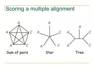
How to generate a multiple alignment? • Given a pairwise alignment, just add the third, then the fourth, and so on!! • dront AGAC • t-rex – – AC • unicorn AG – – • dront AGAC • unicorn AG– – • t-rex – –AC • t-rex AC– – • unicorn AG– – • dront AGAC • t-rex – –AC • unicorn – –AG • A possible general method would be to extend the pairwise alignment method into a simultaneous N-wise alignment, using a complete dynamical-programming algorithm in N dimensions. Algorithmically, this is not difficult to do. • In the case of three sequences to be aligned, one can visualize this reasonable easily: One would set up a three-dimensional matrix (a cube) instead of the two-dimensional matrix for the pairwise comparison. Then one basically performs the same procedure as for the two-sequence case. This time, the result is a path that goes diagonally through the cube from one corner to the opposite. • The problem here is that the time to compute this N-wise alignment becomes prohibitive as the number of sequences grows. The algorithmic complexity is something like O(c2n), where c is a constant, and n is the number of sequences. (See the next section for an explanation of this notation.) This is disastrous, as may be seen in a simple example: if a pairwise alignment of two sequences takes 1 second, then four sequences would take 104 seconds (2.8 hours), five sequences 106 seconds (11.6 days), six sequences 108 seconds (3.2 years), seven sequences 1010 seconds (317 years), and so on. The expected number of hits with score S is:
MML • For a hypothesis H and data D we have from Bayes: • P(H&D) = P(H).P(D|H) = P(D).P(H|D) (1) • P(H) prior probability of hypothesis H • P(H|D) posterior probability of hypothesis H • P(D|H) likelihood of the hypothesis, actually a function of the data given H. • From Shannon's Entropy, the message length of an event E, MsgLen(E), where E has probability P(E), is given by • MsgLen(E) = -log2(P(E)): (2) • From (1) and (2), • MsgLen(H&D) = MsgLen(H)+MsgLen(D|H) = MsgLen(D)+MsgLen(H|D) • Now in inductive inference one often wants the hypothesis H withthe largest posterior probability. max{P(H|D)} • MsgLen(H) can usually be estimated well, for some reasonable prior on hypotheses. MsgLen(D|H) can also usually be calculated. Unfortunately it is often impractical to estimate P(D) which is a pity because it would yield P(H|D). • However, for two rival hypotheses, H and H' • MsgLen(H|D) - MsgLen(H'|D) = MsgLen(H) + MsgLen(D|H) - MsgLen(H') - MsgLen(D|H') = posterior - log odds ratio
Consider a transmitter T and a receiver R connected by one of Shannon's communication channels. T must transmit some data D to R. T and R may have previously agreed on a code book for hypotheses, using common knowledge and prior expectations. If T can find a good hypothesis, H, (theory, structure, pattern, ...) to fit the data then she may be able to transmit the data economically. An explanation is a two part message:(i) transmit H taking MsgLen(H) bits, and (ii) transmit D given H taking MsgLen(D|H) bits. • The message paradigm keeps us "honest": Any information that is not common knowledge must be included in the message for it to be decipherable by the receiver; there can be no hidden parameters.This issue extends to inferring (and stating) real-valued parameters to the "appropriate" level of precision. • The method is "safe": If we use an inefficient code it can only make the hypothesis look less attractive than otherwise.There is a natural hypothesis test: The null-theory corresponds to transmitting the data "as is". (That does not necessarily mean in 8-bit ascii; the language must be efficient.) If a hypothesis cannot better the null-theory then it is not acceptable.
A more complex hypothesis fits the data better than a simpler model, in general. We see that MML encoding gives a trade-off between hypothesiscomplexity, MsgLen(H), and the goodness of fit to the data, MsgLen(D|H). The MML principle is one way to justify and realize Occam's razor. • Continuous Real-Valued Parameters • When a model has one or more continuous, real-valued parameters they must be stated to an "appropriate" level of precision. The parameter must be stated in the explanation, and only a finite number of bits can be used for the purpose, as part of MsgLen(H). The stated value will often be close to the maximum-likelihood value which minimises MsgLen(D|H). • If the -log likelihood, MsgLen(D|H), varies rapidly for small changes in the parameter, the parameter should be stated to high precision. • If the -log likelihood varies only slowly with changes in the parameter, the parameter should be stated to low precision. • The simplest case is the multi-state or multinomial distribution where the data is a sequence of independent values from such a distribution. The hypothesis, H, is an estimate of the probabilities of the various states (eg. the bias of a coin or a dice). The estimate must be stated to an "appropriate" precision, ie. in an appropriate number of bits.
ElementaryProbability • A sample-space (e.g. S={a,c,g,t}) is the set of possible outcomes of some experiment. • Events A, B, C, ..., H, ... An event is a subset (possibly a singleton) of the sample space, e.g. Purine = {a, g}. • Events have probabilities P(A), P(B), etc. • Random variables X, Y, Z, ... A random variable X takes values, with certain probabilities, from the sample space. • We may write P(X=a), P(a) or P({a}) for the probability that X=a. • Thomas Bayes (1702-1761). Bayes'Theorem • If B1, B2, ..., Bkis a partition of a set B (of causes) then • P(Bi|A) = P(A|Bi) P(Bi) / ∑j=1..k P(A|Bj) P(Bj) where i = 1, 2, ..., k • Inference • Bayes theorem is relevant to inference because we may be entertaining a number of exclusive and exhaustive hypotheses H1, H2, ..., Hk, and wish to know which is the best explanation of some observed data D. In that case P(Hi|D) is called the posterior probability of Hi, "posterior" because it is the probability after the data has been observed. • ∑j=1..k P(D|Hj) P(Hj) = P(D) • P(Hi|D) = P(D|Hi) P(Hi) / P(D) --posterior • Note that the Hi can even be an infinite enumerable set. • P(Hi) is called the prior probability of Hi, "prior" because it is the probability before D is known.
Conditional Probability • The probability of B given A is written P(B|A). It is the probability of B provided that A is true; we do not care, either way, if A is false. Conditional probability is defined by: • P(A&B) = P(A).P(B|A) = P(B).P(A|B) • P(A|B) = P(A&B) / P(B), P(B|A) = P(A&B) / P(A) • These rules are a special case of Bayes' theorem for k=2. • There are four combinations for two Boolean variables: • We can still ask what is the probability of A, say, alone • P(A) = P(A & B) + P(A & not B) • P(B) = P(A & B) + P(not A & B)
Independence • A and B are said to be independent if the probability of A does not depend on B and v.v.. In that case P(A|B)=P(A) and P(B|A)=P(B) so • P(A&B) = P(A).P(B) • P(A & not B) = P(A) . P(not B) • P(not A & B) = P(not A).P(B) • P(not A & not B) = P(not A) . P(not B) • A Puzzle • I have a dice (made it myself, so it might be "tricky") which has 1, 2, 3, 4, 5 & 6 on different faces. Opposite faces sum to 7. The results of rolling the dice 100 times (good vigorous rolls on carpet) were: • 1- 20: 3 1 1 3 3 5 1 4 4 2 3 4 3 1 2 4 6 6 6 6 • 21- 40: 3 3 5 1 3 1 5 3 6 5 1 6 2 4 1 2 2 4 5 5 • 41- 60: 1 1 1 1 6 6 5 5 3 5 4 3 3 3 4 3 2 2 2 3 • 61- 80: 5 1 3 3 2 2 2 2 1 2 4 4 1 4 1 5 4 1 4 2 • 81-100: 5 5 6 4 4 6 6 4 6 6 6 3 1 1 1 6 6 2 4 5 • Can you learn anything about the dice from these results? What would you predict might come up at the next roll? How certain are you of your prediction?
Information • Examples • More probable, less information. • I toss a coin and tell you that it came down `heads'. What is the information? A computer scientist immediately says `one bit' (I hope). • {a,c,g,t} information. log2(b^d), base and digits, Codon’s Protein information • Suppose we have a trick coin with two heads and this is common knowledge. I toss the coin and tell you that it came down ... heads. How much information? If you had not known that it was a trick coin, how much information you would have learned, so the information learned depends on your prior knowledge! • Pulling a coin out of my pocket and tell you that it is a trick coin with two heads. How much information have you gained? Well "quite a lot", maybe 20 or more bits, because trick coins are very rare and you may not even have seen one before. • A biased coin; it has a head and a tail but comes down heads about 75 % of the times and tails about 25%, and this is common knowledge. I toss the coin and tell you ... tails, two bits of information. A second toss lands ... heads, rather less than one bit, wouldn't you say? • Information: Definition • The amount of information in learning of an event `A' which has probability P(A) is • I(A) = -log2(P(A)) bits • I(A) = -ln(P(A)) nits (aka nats) • Note that • P(A) = 1 => I(A) = -log2(1) = 0, No information. • P(B) = 1/2 => I(B) = -log2(1/2) = log2(2) = 1 • P(C) = 1/2n => I(C) = n • P(D) = 0 => I(D) = ∞ ... think about it
Entropy • Entropy tells us the average (expected) information in a probability distribution over a sample space S. It is defined to be • H = - ∑v in S {P(v) log2 P(v)} • This is for a discrete sample space but can be extended to a continuous one by the use of an integral. • Examples • The fair coin • H = -1/2 log2(1/2) - 1/2 log2(1/2) = 1/2 + 1/2 = 1 bit • That biased coin, P(head)=0.75, P(tail)=0.25 • H = - 3/4 log2(3/4) - 1/4 log2(1/4) = 3/4 (2 - log2(3)) + 2/4 = 2 - 3/4 log2(3) bits < 1 bit • A biased four-sided dice, p(a)=1/2, p(c)=1/4, p(g)=p(t)=1/8 • H = - 1/2 log2(1/2) - 1/4 log2(1/4) - 1/8 log2(1/8) - 1/8 log2(1/8) = 1 3/4 bits
Theorem H1 (The result is "classic" but this is from notes taken during talks by Chris Wallace (1988).) http://www.csse.monash.edu.au/~lloyd/tildeMML/Notes/Information/ • If (pi)i=1..N and (qi)i=1..N are probability distributions, i.e. each non-negative and sums to one, then the expression • ∑1=1..N { - pi log2(qi) } is minimized when qi=pi • Proof: First note that to minimize f(a,b,c) subject to g(a,b,c)=0, we consider f(a,b,c)+λ.g(a,b,c). We have to do this because a, b & c are not independent; they are constrained by g(a,b,c)=0. If we were just to set d/da{f(a,b,c)} to zero we would miss any effects that `a' has on b & c through g( ). We don't know how important these effects are in advance, but λ will tell us.We differentiate and set to zero the following: d/da{f(a,b,c)+λ.g(a,b,c)}=0 and similarly for d/db. d/dc and d/dλ. • d/d dwi { - ∑j=1..N pj log2 wj + λ((∑j=1..N wj) - 1) } = - pi/wi + λ = 0 • hence wi = pi / λ • ∑ pi = 1, and ∑ wi = 1, so λ = 1 • hence wi = pi • Corollary (Information Inequality) • ∑i=1..N { pi log2( pi / qi) } ≥ 0 • with equality iff pi=qi, e.g., see Farr (1999).
Kullback-Leibler Distance • The left-hand side of the information inequality • ∑i=1..N { pi log2( pi / qi) } • is called the Kullback-Leibler distance (also relative entropy) of the probability distribution (qi) from the probability distribution (pi). It is always non-negative. Note that it is not symmetric in general. (The Kullback-Leibler distance is defined on continuous distributions through the use of an integral in place of the sum.) • Exercise • Calculate the Kullback Leibler distances between the fair and biased (above) probability distributions for the four-sided dice. • Notes • S. Kullback & R. A. Leibler. On Information and Sufficiency. Annals of Math. Stats. 22 pp.79-86 1951 • S. Kullback. Information Theory and Statistics. Wiley 1959 • C. S. Wallace. Information Theory. Dept. Computer Science, Monash University, Victoria, Australia, 1988 • G. Farr. Information Theory and MML Inference. School of Computer Science and Software Engineering, Monash University, Victoria, Australia, 1999
Inference, Introduction • People often distinguish between • selecting a model class • selecting a model from a given class and • estimating the parameter values of a given model • to fit some data. • It is argued that although these distinctions are sometimes of practical convenience, that's all: They are all really one and the same process of inference. • A (parameter estimate of a) model (class) is not a prediction, at least not a prediction of future data, although it might be used to predict future data. It is an explanation of, a hypothesis about, the process that generated the data. It can be a good explanation or a bad explanation. Naturally we prefer good explanations. • Model Class • e.g. polynomial models form a model class for sequences of points {<xi,yi>} s.t. xi<xi+1}. The class includes constants, straight lines, quadratics, cubics, etc. and note that these have increasing numbers of parameters; they grow more complex. (Note also that the class does not include functions based on trigonometric functions; since they form another class). • Model • e.g. The general cubic equation y = ax3+bx2+cx+d is a model for {<xi,yi>} s.t. xi<xi+1}. It has four parameters a, b, c & d which can be estimated to fit the model to some given data. • It is usually the case that a model has a fixed number of parameters (e.g. four above), but this can become blurred if hierarchical parameters or dependent parameters crop up. • Some writers reserve `model' for a model (as above) where all the parameters have fixed, e.g. inferred, values; if there is any ambiguity I will (try to) use model instance for the latter. e.g. The normal distribution N(μ,σ) is a model and N(0,1) is a model instance. • Parameter Estimation • e.g. If we estimate the parameters of a cubic to be a=1, b=2, c=3 & d=4, we get the particular cubic polynomial y = x3+2x2+3x+4.
Inference Hypothesis Complexity • Over-fitting • Over-fitting often appears as selecting a too complex model for the data. e.g. Given ten data points from a physics experiment, a 9th-degree polynomial could be fitted through them, exactly. This would almost certainly be a ridiculous thing to do. That small amount of data is probably better described by a straight line or by a quadratic with any minor variations explained as "noise" and experimental error. • Parameter estimation provides another manifestation of over-fitting: stating a parameter value too accurately is also over-fitting. • e.g. I toss a coin three times. It lands `heads' once and `tails' twice. What do we infer? p=0.5, p=0.3, p=0.33, p=0.333 or p=0.3333, etc.? In fact we learn almost nothing, except that the coin does have a head on one side and a tail on the other; p>0 and p<1. • e.g. I toss a coin 30 times. It lands `heads' 10 times and `tails' 20 times. We are probably justified in starting to suspect a bias, perhaps 0.2<p<0.4. • The accuracy with which the bias of a coin can be estimated can be made precise; see the [2-State / Binomial Distribution]. • Classical statistics has developed a variety of significance tests to judge whether a model is justified by the data. An alternative is described below.
Inference: MML • Attempts to minimise the discrepancy between given data, D, and values implied by a hypothesis, H, almost always results in over-fitting, i.e. a too complex hypothesis (model, parameter estimate,...). e.g. If a quadratic gives a certain root mean squared (RMS) error, then a cubic will in general give a smaller RMS value. • Some penalty for the complexity of H is needed to give teeth to the so-called "law of diminishing returns". The minimum message length (MML) criterion is to consider a two-part message (remember [Bayes]): • 2-part message: H; (D|H) • probabilities: P(H&D) = P(H).P(D|H) • message length: msgLen(H&D) = msgLen(H) + msgLen(D|H) • A complex hypothesis has a small prior probability, P(H), a large msgLen(H); it had better make a big saving on msgLen(D|H) to pay for its msgLen(H). The name `minimum message length' is after Shannon's mathematical theory of communication. • The first part of the two-part message can be considered to be a "header", as in data compression or data communication. Many file compression algorithms produce a header in the compressed file which states a number of parameter values etc., which are necessary for the data to be decoded. • The use of a prior, P(H), is considered to be controversial in classical statistics. • Notes • The idea of using compression to guide inference seems to have started in the 1960s. • R. J. Solomonoff. A Formal Theory of Inductive Inference, I and II. Information and Control 7 pp1-22 and pp224-254, 1964 • A. N. Kolmogorov. Three approaches to the Quantitaive Definition of Information. Problems of Information and Transmission 1(1) pp1-7, 1965 • G. J. Chaitin. On the Length of Programs for Computing Finite Binary Sequences. JACM 13(4) pp547-569, Oct' 1966 • C. S. Wallace and D. M. Boulton. An Information Measure for Classification. CACM 11(2) pp185-194, Aug' 1968
Inference: More Formally • Theta: variously the parameter-space, model class etc. • theta or H: variously a particular parameter value, hypothesis, model, etc • P(theta) or P(H): prior probability of parameter value, hypothesis etc. • X: data space, set of all possible observations • D: data, an observation, D:X, often x:X • P(D|H): the likelihood of the data D, is also written as f(D|H) • P(H|D) or P(theta|D): the posterior probability of an estimate or hypothesis etc. given observed data • P(D, H) = P(D & H): joint probability of D and H • m(D) :X->Theta, function mapping observed data D onto an inferred parameter estimate, hypothesis, etc. as appropriate • Maximum Likelihood • The maximum likelihood principle is to choose H so as to maximize P(D|H) e.g. Binomial Distribution (Bernouilli Trials) • A coin is tossed N times, landing heads, #head-times, and landing `tails', #tail=N-#head times. We want to infer p=P(head). The likelihood of <#head,#tail> is: • P(#head|p) = p#head.(1-p)#tail • Take the -ve log because (it's easier and) maximizing the likelihood is equivalent to minimizing the negative log likelihood: • - log2(P(#head|p)) = -#head.log2(p) -#tail.log2(1-p)
- log2(P(#head|p)) = -#head.log2(p) -#tail.log2(1-p) • differentiate with respect to p and set to zero: • -#head/p + #tail/(1-p) = 0 • #head/p = #tail/(1-p) • #head.(1-p) = (N-#head).p • #head = N.p • p = #head / N, q = 1-p = #tail / N • So the maximum-likelihood inference for the bias of the coin is #head/N. • To sow some seeds of doubt, note that if the coin is thrown just once, the estimate for p must be either 0.0 or 1.0, which seems rather silly, although one could argue that such a small number of trials is itself rather silly. Still, if the coin were thrown 10 times and happened to land heads 10 times, which is conceivable, an estimate of 1.0 is not sensible. • e.g. Normal Distribution • Given N data points, the maximum likelihood estimators for the parameters of a normal distribution, μ', σ' are given by: • μ' = {∑i=1..N xi} / N --the sample mean • σ'2 = ∑i=1..N (xi - μ')2} / N --the sample variance • Note that σ'2 is biased, e.g. if there are just two data values it is implicitly assumed that they lie on opposite sides of the mean which plainly is not necessarily the case, i.e. the variance is under-estimated. • Notes • This section follows Farr (p17..., 1999) • G. Farr. Information Theory and MML Inference. School of Computer Science and Software Engineering, Monash University, 1999
HMM (PFSM) • A Markov Model is a probabilistic process defined over a finite sequence of events – or states; (s_1, …, s_n), the probability of each of which depends only on the events proceeding. Each state-transition generates a character from the alphabet of the process. The probability of a sequence x with a certain pattern appearing next, in a given state S(j), pr(x(t)=S(j)), may depend on the prior history of t-1 events. • Probabilistic Finite State Automata (PFSA) or Machine. • Order of the model is the length of the history, or the context upon which the probabilities of the next outcome depends on. • 0th order has no dependency to the past pr{x(t) = S(i)} = pr{x(t‘) = S(j)}. • 2nd order depends upon the two previous states pr{x(t) = S(j)} | { pr{x(t-1) = S(m), pr{x(t-2) = S(n) }}, for I,m,n = 1..k. • A Hidden Markov Model (HMM) is an MM but the states are hidden. For example, in the case of deleted genetic sequences where nucleotide density information is lost, or neither the architecture of the model nor the transitions are known - hidden. • One must search for an automaton that explains the data well (pdf). • It is necessary to weigh the trade-off between the complexity of the model and its fit to the data.
a Hidden Markov Model (HMM) represents stochastic sequences as Markov chains where the states are not directly observed, but are associated with a pdf. The generation of a random sequence is then the result of a random walk in the chain (i.e. the browsing of a random sequence of states S = {s1; sn} and the result of a draw (called an emission) at each visit of a state. • The sequence of states, which is the quantity of interest in most of the pattern recognition problems, can be observed only through the stochastic processes defined into each state (i.e. before being able to associate a set of states to a set of observations, the parameters of the pdfs of each state must be known. The true sequence of states is therefore hidden by a first layer of stochastic processes. HMMs are dynamic models, in the sense that they are specifically designed to account for some macroscopic structure of the random sequences. Consider random sequences of observations as the result of a series of independent draws in one or several Gaussian densities. To this simple statistical modeling scheme, HMMs add the specification of some statistical dependence between the (Gaussian) densities from which the observations are drawn.
Frequency or counts n = 1000 n = 2 Match Score • Assessing significance requires a distribution • I have an apple of diameter 5”. How unusual? • Is a match significant? • Depends on: • Scoring system • Database • Sequence to search for • *** Length • *** Composition • How do we determine therandom sequences? • Generating “random” sequences • Random uniform model: P(G) = P(A) = P(C) = P(T) = 0.25 • Doesn’t reflect nature • Use sequences from a database • Might have genuine homology • ?? We want unrelated sequences • Random shuffling of sequences • Preserves composition • Removes true homology What distribution do we expect to see? The mean of n random (i.i.d.) events tends towards a Gaussian distribution. Example: Throw n dice and compute the mean. Distribution of means:
The extreme value distribution • This means that if we get the match scores for our sequence with n other sequences, the mean would follow a Gaussian distribution. • The maximum of n (i.i.d.) random events tends towards the extreme value distribution as n grows large. Gaussian: Extreme Value:

