Bayesian estimation Why and How to Run Your First Bayesian Model
800 likes | 966 Views
Bayesian estimation Why and How to Run Your First Bayesian Model. Rens van de Schoot Rensvandeschoot. com. Classical null hypothesis testing. Wainer: "One Cheer for Null-Hypothesis Significance Testing“ (1999; Psych. Meth., 4 , 212-213) … however …. NHT vs. Bayes.

Bayesian estimation Why and How to Run Your First Bayesian Model
E N D
Presentation Transcript
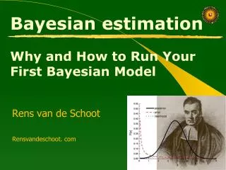
Bayesian estimation Why and How to Run Your First Bayesian Model Rens van de Schoot Rensvandeschoot. com
Classical null hypothesis testing Wainer: "One Cheer for Null-Hypothesis Significance Testing“ (1999; Psych. Meth., 4, 212-213) … however …
NHT vs. Bayes Pr (Data | H0) ≠ Pr (Hi | Data)
Bayes Theorem • Pr (Hi | Data) = • Posterior ≈ prior * data • Posterior probability is proportional to the product of the prior probability and the likelihood
Bayes theorem: prior, data and posterior Bayes Theorem:
Bayes Theorem • Pr (Hi| Data) = • Posterior ≈ prior * data • Posterior probability is proportional to the product of the prior probability and the likelihood
Intelligence (IQ) -∞ ∞ IQ
Prior Knowledgde 1 -∞ ∞ IQ
Prior Knowledgde IQ 40 180
Prior Knowledgde 2 IQ 40 180
Prior Knowledgde 3 100 40 180 IQ
Prior Knowledgde 4 100 40 180 IQ
Prior Knowledgde 5 100 40 180 IQ
Prior Knowledgde 1 -∞ ∞ 2 3 5 4
Prior Prior -∞ ∞ IQ
Data Data Prior -∞ ∞ IQ
Posterior Posterior Data Prior -∞ ∞ IQ
Prior - Data Data Prior 100 40 180 IQ
Prior - Data Data Prior 100 40 180 IQ
How to obtain posterior? • In complex models, the posterior is often intractable (impossible to compute exactly) • Solution: approximate posterior by simulation • Simulate many draws from posterior distribution • Compute mode, median, mean, 95% interval et cetera from the simulated draws
ANOVAexample 4 unknown parameters μj (j=1,...,4) and one common but unknown σ2. Statistical model: Y = μ1*D1 + μ2*D2 + μ3*D3 + μ4*D4 + E with E ~ N(0, σ2)
The Gibbs sampler Specify prior: Pr(μ1, μ2, μ3, μ4, σ2) Prior (μj) ~ Nor(μ0, var0) Prior (μj) ~ Nor(0,10000) Prior (σ2) ~ IG(0.001, 0.001)
Prior is Inverse Gamma a (shape), b (scale)
The Gibbs sampler Combine prior with likelihood provides posterior: Post ( μ1, μ2, μ3, μ4, σ2 | data ) …this is a 5 dimensional distribution…
The Gibbs sampler • Iterative evaluation via conditional distributions: • Post ( μ1 | μ2, μ3, μ4, σ2, data ) ~ Prior (μ1) X Data (μ1) • Post ( μ2 | μ1, μ3, μ4, σ2, data ) ~ Prior (μ2) X Data (μ2) • Post ( μ3 | μ1, μ2, μ4, σ2, data ) ~ Prior (μ3) X Data (μ3) • Post ( μ4 | μ1, μ2, μ3, σ2, data ) ~ Prior (μ4) X Data (μ4) • Post ( σ2 | μ1, μ2, μ3, μ4, data ) ~ Prior (σ2) X Data (σ2)
The Gibbs sampler • Assign starting values • Sample μ1 from conditional distribution • Sample μ2 from conditional distribution • Sample μ3 from conditional distribution • Sample μ4 from conditional distribution • Sample σ2 from conditional distribution • Go to step 2 until enough iterations
Burn In • Gibbs sampler must run t iterations ‘burn in’ before we reach target distribution f(Z) • How many iterations are needed to converge on the target distribution? • Diagnostics • Examine graph of burn in • Try different starting values • Run several chains in parallel
Conclusion about convergenge • Burn-in: Mplus deletes first half of chain • Run multiple chains (Mplus default 2) • Decrease Bconvergence: default .05 but better use .01 • ALWAYS do a graphical evaluation of each and every parameter
Summing up • Degree of belief • What is known before observing the data • What is known after observing the • Tool to include subjective knowledge • Try to express absence of prior knowledge • Posterior mainly determined by data • Simulation (sampling) techniques to obtain the posterior distribution and all posterior summary measures • Important to check • Probability • Prior • Posterior • Informative prior • Non-informative prior • MCMC methods • Convergence
IQ • N = 20 • Data are generated • Mean = 102 • SD = 15 • N = 20 • Data are generated • Mean = 102 • SD = 15 IQ
Technical Intermezzo ...C.C.I.??? 43 43
Uncertainty in Classical Statistics • Uncertainty = sampling distribution • Estimate population parameter by • Imagine drawing an infinity of samples • Distribution of over samples • Problem is that we have only one sample • Estimate and its sampling distribution • Estimate 95% confidence interval
Inference in Classical Statistics • What does 95% confidence interval actually mean? • Over an infinity of samples, 95% of these contain the true population value • But we have only one sample • We never know if our present estimate and confidence interval is one of those 95% or not
Inference in Classical Statistics • What does 95% confidence interval NOT mean? • We have a 95% probability that the true population value is within the limits of our confidence interval • We only have an aggregate assurance that in the long run 95% of our confidence intervals contain the true population value
Uncertainty in Bayesian Statistics • Uncertainty = probability distribution for the population parameter • In classical statistics the population parameter has one single true value • In Bayesian statistics we imagine a distribution of possible values of population parameter
Inference in Bayesian Statistics • What does a95% central credibility interval mean? • We have a 95% probability that the population value is within the limits of our confidence interval
What have we learned so far? • Results are compromise of prior & data • However: • -> non/low-informative priors • -> informative priors • -> misspecification of the prior • -> convergence • Results are easier to communicate • (eg CCI compared to confidence interval)
Software • WinBUGS/ OpenBUGS • Bayesian inference Using Gibbs Sampling • Very general, user must set up model • R packages • LearnBayes, R2Winbugs, MCMCpack • MLwiN • Special implementation for multilevel regression • AMOS • Special implementation for SEM • Mplus • Very general (SEM + ML + many other models)