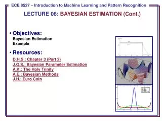
LECTURE 06: BAYESIAN ESTIMATION (Cont.)
LECTURE 06: BAYESIAN ESTIMATION (Cont.). • Objectives: Bayesian Estimation Example Resources: D.H.S.: Chapter 3 (Part 2) J.O.S.: Bayesian Parameter Estimation A.K.: The Holy Trinity A.E.: Bayesian Methods J.H.: Euro Coin. The Parameter Distribution.

LECTURE 06: BAYESIAN ESTIMATION (Cont.)
E N D
Presentation Transcript
LECTURE 06: BAYESIAN ESTIMATION (Cont.) • Objectives:Bayesian EstimationExample • Resources: • D.H.S.: Chapter 3 (Part 2)J.O.S.: Bayesian Parameter EstimationA.K.: The Holy TrinityA.E.: Bayesian MethodsJ.H.: Euro Coin
The Parameter Distribution • Assume the parametric form of the evidence, p(x), is known: p(x|θ). • Any information we have about θprior to collecting samples is contained in a known prior density p(θ). • Observation of samples converts this to a posterior, p(θ|D), which we hope is peaked around the true value ofθ. • Our goal is to estimate a parameter vector: • We can write the joint distribution as a product: because the samples are drawn independently. • This equation links the class-conditional density to the posterior, . But numerical solutions are typically required!
Case: only mean unknown • Known prior density: Univariate Gaussian Case • Using Bayes formula: • Rationale: Once a value of μ is known, the density for x is completely known. αis a normalization factor that depends on the data, D.
Univariate Gaussian Case • Applying our Gaussian assumptions:
Univariate Gaussian Case (Cont.) • Now we need to work this into a simpler form:
Univariate Gaussian Case (Cont.) • p(μ|D) is an exponential of a quadratic function, which makes it a normal distribution. Because this is true for any n, it is referred to as a reproducing density. • p(μ)is referred to as a conjugate prior. • Write p(μ|D) ~ N(μn,σn2): • Expand the quadratic term: • Equate coefficients of our two functions:
Univariate Gaussian Case (Cont.) • Rearrange terms so that the dependencies on μ are clear: • Associate terms related to σ2and μ: • There is actually a third equation involving terms not related to μ: • but we can ignore this since it is not a function of μ and is a complicated equation to solve.
Univariate Gaussian Case (Cont.) • Two equations and two unknowns. Solve for μnand σn2. First, solve for μn2 : • Next, solve for μn: • Summarizing:
Summary • Introduction of Bayesian parameter estimation. • The role of the class-conditional distribution in a Bayesian estimate. • Estimation of the posterior and probability density function assuming the only unknown parameter is the mean, and the conditional density of the “features” given the mean, p(x|θ), can be modeled as a Gaussian distribution. • Bayesian estimates of the mean for the multivariate Gaussian case. • General theory for Bayesian estimation. • Comparison to maximum likelihood estimates. • Recursive Bayesian incremental learning. • Noninformative priors. • Sufficient statistics • Kernel density.
“The Euro Coin” • Getting ahead a bit, let’s see how we can put these ideas to work on a simple example due to David MacKay, and explained by Jon Hamaker.