Disk-Covering Method
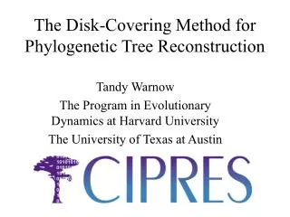
Orangutan. Human. Gorilla. Chimpanzee. Disk-Covering Method. From the Tree of the Life Website, University of Arizona. Based on the paper by D.Huson, S.Nettles, T.Warnow. Presented by Galiya S. , Eduard S. Phylogenetic Tree. From the Desert Vista high school, Phoenix, Arizona.


Disk-Covering Method
E N D
Presentation Transcript
Orangutan Human Gorilla Chimpanzee Disk-Covering Method From the Tree of the Life Website,University of Arizona Based on the paper by D.Huson, S.Nettles, T.Warnow Presented by Galiya S. , Eduard S.
Phylogenetic Tree From the Desert Vista high school, Phoenix, Arizona A phylogenetic tree is a tree showing the evolutionary interrelationships among various species.
AGGCCT GGACTT 3. The sites evolve identically and independently (i.i.d) down the tree from the root. Jukes-Cantor model • Definition 1: Let T be a fixed rooted tree with leaves labeled 1,…,n. • The Jukes-Cantor model makes the following assumptions: • The possible states for each site are A,C,T,G. • 2. The sequence length is an input parameter and for each site, the state at the root is drawn from a distribution (typically uniform). site AGACTT
u AGACTT e v AGGCCT GGACTT GGGCAT AGCCCT GCACTT Jukes-Cantor model (cont.) 4. For each edge with u the parent of v, if thestate of asite is different at u than at v, then the probability that v has any state of the three remaining states is equal. The example above based on CIPRES ppt. University of Texas at Austin.
AGTCTG • Multiple changes at a single site – hidden changes:seq1 AGTCAGseq2 AGTCAC • Number of changes: Seq1TGCA • Seq2TA AGTCAG AGTCAC 1 2 3 1 Jukes-Cantor model (cont.) 5.To each edge e in the tree T associated a Poisson random variable for the number of mutations of a randomly selectedsite on that edge. 6. Each edge has an expectancy , .
e • Definition 2: T is the unrooted true tree, and T’ is the unrooted inferred tree, both with leaves labeled 1,…,n. e is internal edge. let define: Definition 2 • split- Removing an edge e from an unrooted phylogenetic tree T partitions the leaf set S of the tree into two not empty sets. We denote it . Example: 5 T: 1 4 2 3 S={1,2,3,4,5}
5 Example: e2 1 e1 FN 4 2 3 3 4 1 e2 e1 FP 2 5 Definition 2 (cont.) • Any split is called a false negative (FN). • Any split is called a false positive (PN). • An edge is recovered in T’ if the split appears in . T: T’:
5 Example: e2 e1 T: 1 FN 4 2 FN=0.5=50% FP=0.5=50% 3 4 T’: 3 1 e2 e1 FP 2 5 Definition 2 (cont.) • FP rate: • FN rate:
Additive matrix • Definition 3: A matrix D is called additive if there exists a tree T with positive edge weighting w such that . is the path in T between leaves i and j. • Given an additive matrix D the tree T can be uniquely reconstruct in . • A dissimilarity matrix is a symmetric matrix that is 0 on the diagonal.
remainder: Let T be the unrooted true tree. is the path in T between leaves i and j. we represent the evolutionary process by a set of Poisson process. True distance i Xe1 Xe2 Xe3 j Xij= Xe1+Xe2+Xe3 • is called the true distance between i and j. • is an additive matrix.
is the sequence length. • is the normalized Hamming distance. Hamming Distance • is the number of different sites between sequences i and j. is called the Hamming Distance. • Example: s1CAACCCCGGT H(s1, s2) =4 s2 TAATTTCGGT k = 10 h(s1, s2) =4/10= 0.4
If : 1 3 TTGCC • The 4 leaves are: TCAAG 2 4 TGGCC TTGGA Replace * with 0.778 * distance correction • Jukes-Cantor distance correctionfor each two leavesi, jis: • Afterwards, compute the maximum Jukes-Cantor distance,multiplythatvalue by the number n of leaves and replace all undefined values. • Example: • The matrix d is:
Example: q=3.2 0 1.2 2.8 3 1 0 3.1 0 0 1.1 0 0 1.5 0 0 0.2 0 0.2 0.3 0 0 0.4 0 The error • Definition 7: Let be a real number. Then: and
2 4 1 Threshold Graph Let d be an dissimilarity matrix and let be any real number. The thresholdgraph Thresh(d,q) is defined as: Vertex set is {1,2,…,n }. The edges are: (i,j) is an edge if and only if q. For example: q = 4.5 Thresh(d,4.5):
Triangulated graph Definetion: A graph is triangulated if no subset of nodes induced a cycle of size four or more. Taken from wikipedia
Disk Covering Method • A generic disk-covering method has four steps: • Decomposition: Compute a decomposition of the dataset into overlapping subsets. • Solution: Construct trees on the subsets using a base method. • Merge: Use a supertree method to merge the trees on the subsets into a tree on the full dataset. • 4. Refinement: Compute the asymetric mediantree of all posible supertrees. The example above based on CIPRES ppt. University of Texas at Austin.
Simplicial elimination order Lemma: Simplicial elimination order is ordering of the vertices of G so the set Form a clique. Every triangulated graph G has a simplicial elimination ordering. The maximal clique in G are of the form This ordering can be found at . So maximal cliques of G can be found at Example: 5 3 7 8
Constructing Tq input: d dissimilarity matrix, Real number q>0. output: reconstructed tree, Tq. 1. Compute Thresh(d,q) 2. Triangulate Thresh(d,q) Polynomial Complexity 3. Compute Buneman Trees far all Maximal Cliques in Triangulated Thresh(d,q). 4. Merge subtrees into a supertree. Overall Complexity: Polynomial Complexity
Intersection graph Intersection graph is undirected graph formed by sets of sets of vertices: by choosing one vertex for each set and connecting two vertices when the corresponding sets have none empty intersection. Taken from wikipedia
tree T’ subtree of T’ Triangulaing Tresh(d,q) Complexity Lemma: If d is an additive matrix, then Tresh(d,q) is triangulated. Proof: let d be an arbitrary additive matrix, and let (T,w) be the edge weighted tree associated uniquily to d. Let q > 0. Add intermediate vertices to the edges of T and re-weight the edges so that the path between leaf pair are unchanged, but for every pair of leaves u and v in T if then there is a node x in the enlarged tree T’ so that
tree T Triangulaing Tresh(d,q) Complexity Now let denote the subtree of T’ of distance at most q/2 of u. Note that if only if , and so the Thresh(d,q) is identical to the intersection graph of the as u ranges over the leaves of T. Consecuntly Thresh(d,q) is triangulated. Intersection Graph Thresh(d,q) Taken from wikipedia
Supertree Construction Algorithm (SCA) Step 1 : First obtain a simplicial elemination ordering for G. Compute where For each Ci find a maximal clique C containing Ci and compute a tree ti for Ci by deleting the leaves in C-Ci form Tc. Step 2 : Construct tree for i = n-3,n-4,…,1 compute the tree Ti formed by merging ti and using Consensus Subtree Merger method Example: C: {1,2,3,4} C2: { 2,3,4} C-C2{1 } left { 2,3,4}
1 2 1 2 3 3 2 5 5 4 4 6 2 1 1 6 1 2 1 2 3 3 4 4 7 3 3 4 4 7 Strict Consenseus Subtree Merger This method contracts a minimum set of edges in each tree in order to make them identical on the subtree they induce, lets denote that subtree by X and call it the backbone. Merging two tree is done by attaching the pieces of each tree appropriately to the different edges of the backbone. The situatuion in which the some piece of each tree attaches onto the same edge of the backbone, called collision.
subtree of A subtree of B a e b subtree of D subtree of C d c Short Quartet Definition Let (T,w) be a binary tree edge weighted by , and leaf laled by the set of spieces. Let e be an edge in T that is not incident to a leaf of T. Aroun e there is four subtrees A,B,C,D. Let a,b,c,d be four laves of the subtrees A,B,C,D repectivly, closest to e.Where the distance between leaves i and j measured as . We call {a,b,c,d} a short quartet around e. and the collection of all short quartets around internal nodes of T is denoted by
j i Gsq Definition Let be the additive distance matrix associated to T. The Graph Gsq on the vertex set S = {1,2,…,n} is defined by if i and j are in same short quatet Examples: T j i
Proof of Tq correctness Theorem: Let T be a leaf-labeled tree, Let G be a triangulated graph such that . Let Be the collection of Buneman trees applied to on the maximal cliques of G and assume this collection reconstructs the correct subtree, and let T* be the tree obtained by applying SCA to (G, ). Then T*=T. Proof: We will show that under this conditions, Ti and the T restricted to the same vertices are identical and no collision occur. Part I: Let T be a tree whose leaves are labeled by . Let G be a triangulated graph on S, and let where is a tree on leaf set A for every maximal clique A in G. Let be a simplicial elimination ordering of G. Let show that for every i Base: this is true since we assumed that all buneman trees are correct.
Proof of Tq correctness(Cont.) Lets assume for some . forms the leaf set of the back bone of the strict consensus merger of . So we get Consequently there is no edge contraction when we compute the back bone. Part II: There can be a collision only if the backbone contains an edge onto which both and some other attach, denote this edge by e. Thus, some subtree t’ of Ti attached onto e. Let the leaf set of t’ by . Let P be a path in T corresponding to edge e and let its endpoints be a and b. Let denote T0 be subtree of T obtained by deleting all the nodes in T that are separated from a by the deletion of b, and vice versa. Let be the leaves of T0. The following are true: 1. and all leaves in t’ are also in 2. restricted to is path connected. 3.
Proof of Tq correctness(Cont.) Now, let P’ be a path lying in form to some node in Y. Let y be the first node in Y on the path P’. by (3) also lies entirely in so Consequently But this contradicts earlier assumption that
Experimental Results-Buneman • FN rate of DCM-Buneman is lower than Buneman for every sequnce length. • FP rate of DCM-Buneman is slightly higher than Buneman 3% and 0% respectively • FN rate of DCM-Buneman reaches 5% at 10,000 sequence length,Buneman doesn’t reach this value.
Experimental Results - NJ • FN and FP rates of DCM-NJ is significantly lower than NJ. • DCM-NJ becomes lower then 5% at 250 sequence length. • DCM-NJ can reconstruct the true tree at sequence beyond length of 900.
Distance Methods • A distance matrix D is a symmetric, non-negative with zero diagonal. • The goal is a phylogenetic tree T such that the distance between species in T approximate The distance in D. • we now describe some distance methods.
i k i k e j j l l ij | kl star Buneman • Input:a dissimilarity matrix d. • Output:tree T. • 1. Topology on every four-leaf subset is inferred usingFour-Point Method: Input – 4*4 dissimilarity matrix on i, j ,k, l. Output – • if dij+dkl< min {dik+djl, dil+djk} then: The topology ij | kl (i, j are separated from k, lby an edge) is returned. • ifdij+dkl= min {dik+djl, dil+djk} then a star tree is returned.
4 4 4 1 1 2 5 5 5 2 3 3 1,2 | 4,5 1,3 | 4,5 2,3 | 4,5 Buneman (cont.) • Let Q be a set of four-leaf trees, defined by the FPM. • The buneman tree is the maximally resolved tree satisfying: • for all quartets i, j, k, l if T restricted to i, j, k, l induces a binary tree, then: the tree in Q in i, j, k, l is the same binary tree. • Lemma 1: Let d be an input dissimilarity matrix. Let T be the buneman tree defined by d. Then C(T) is the set of splits (A, B) defined by: • complexity: polynomial time. A={1,2,3} B={4,5} Q: C(T)={(A,B)}
Neighbor - Joining • Input: a distance matrix d. • Output: unrooted binary tree T. • Algorithm Description: • For every 2 species, it determines a score, based on the distance matrix. • At each step the algorithm joins the pair with the minimum score: make a subtree whose root replaces the two chosen species in the matrix. • The distance are recalculated to this new node. • This is reapeted until only tree nodes remain. • Finally, it connects the remaining two vertices with edge. • complexity: polynomial time - o(n3)