The Disk-Covering Method for Phylogenetic Tree Reconstruction
690 likes | 889 Views
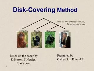
The Disk-Covering Method for Phylogenetic Tree Reconstruction. Tandy Warnow The Program in Evolutionary Dynamics at Harvard University The University of Texas at Austin. Phylogeny. From the Tree of the Life Website, University of Arizona. Orangutan. Human. Gorilla. Chimpanzee.

The Disk-Covering Method for Phylogenetic Tree Reconstruction
E N D
Presentation Transcript
The Disk-Covering Method for Phylogenetic Tree Reconstruction Tandy Warnow The Program in Evolutionary Dynamics at Harvard University The University of Texas at Austin
Phylogeny From the Tree of the Life Website,University of Arizona Orangutan Human Gorilla Chimpanzee
Evolution informs about everything in biology • Big genome sequencing projects just produce data – so what? • Evolutionary history relates all organisms and genes, and helps us understand and predict • interactions between genes (genetic networks) • drug design • predicting functions of genes • influenza vaccine development • origins and spread of disease • origins and migrations of humans
Reconstructing the “Tree” of Life Handling large datasets: millions of species
Cyber Infrastructure for Phylogenetic Research Purpose: to create a national infrastructure of hardware, algorithms, database technology, etc., necessary to infer the Tree of Life. Group: 40 biologists, computer scientists, and mathematicians from 13 institutions. Funding: $11.6 M (large ITR grant from NSF).
-3 mil yrs AAGACTT AAGACTT -2 mil yrs AAGGCCT AAGGCCT AAGGCCT AAGGCCT TGGACTT TGGACTT TGGACTT TGGACTT -1 mil yrs AGGGCAT AGGGCAT AGGGCAT TAGCCCT TAGCCCT TAGCCCT AGCACTT AGCACTT AGCACTT today AGGGCAT TAGCCCA TAGACTT AGCACAA AGCGCTT AGGGCAT TAGCCCA TAGACTT AGCACAA AGCGCTT DNA Sequence Evolution
Phylogeny Problem U V W X Y AGGGCAT TAGCCCA TAGACTT TGCACAA TGCGCTT X U Y V W
Local optimum Cost Global optimum Phylogenetic trees Phylogenetic reconstruction methods • Hill-climbing heuristics for hard optimization criteria (Maximum Parsimony and Maximum Likelihood) • Polynomial time distance-based methods: Neighbor Joining, FastME, Weighbor, etc.
Performance criteria • Running time. • Space. • Statistical performance issues (e.g., statistical consistency) with respect to a Markov model of evolution. • “Topological accuracy” with respect to the underlying true tree. Typically studied in simulation. • Accuracy with respect to a particular criterion (e.g. tree length or likelihood score), on real data.
Markov models of site evolution Simplest (Jukes-Cantor): • The model tree is a pair (T,{e,p(e)}), where T is a rooted binary tree, and p(e) is the probability of a substitution on the edge e • The state at the root is random • If a site changes on an edge, it changes with equal probability to each of the remaining states • The evolutionary process is Markovian More complex models (such as the General Markov model) are also considered, with little change to the theory. Variation between different sites is either prohibited or minimized, in order to ensure identifiability of the model.
Maximum Parsimony • Input: Set S of n aligned sequences of length k • Output: • A phylogenetic tree T leaf-labeled by sequences in S • additional sequences of length k labeling the internal nodes of T such that is minimized.
Maximum Likelihood • Input: Set S of n aligned sequences of length k, and a specified parametric model • Output: • A phylogenetic tree T leaf-labeled by sequences in S • With additional model parameters (e.g. edge “lengths”) such that Pr[S|(T, params)] is maximized.
Local optimum Cost Global optimum Phylogenetic trees Approaches for “solving” MP/ML • Hill-climbing heuristics (which can get stuck in local optima) • Randomized algorithms for getting out of local optima • Approximation algorithms for MP (based upon Steiner Tree approximation algorithms).
Theoretical results • Neighbor Joining is polynomial time, and statistically consistent under typical models of evolution. • Maximum Parsimony is NP-hard, and even exact solutions are not statistically consistent under typical models. • Maximum Likelihood is of unknown computational complexity, but statistically consistent under typical models.
Quantifying Error FN FN: false negative (missing edge) FP: false positive (incorrect edge) 50% error rate FP
Neighbor joining has poor performance on large diameter trees [Nakhleh et al. ISMB 2001] Simulation study based upon fixed edge lengths, K2P model of evolution, sequence lengths fixed to 1000 nucleotides. Error rates reflect proportion of incorrect edges in inferred trees. 0.8 NJ 0.6 Error Rate 0.4 0.2 0 0 400 800 1200 1600 No. Taxa
Theoretical convergence rates • Atteson: Let T be a model tree defining additive matrix D. Then Neighbor Joining will reconstruct the true tree with high probability from sequences that are of length at least O(lg n emax Dij). • Proof: Show NJ accurate on input matrix d such that max{|Dij-dij|}<f/2, for f the minimum edge length.
Other standard polynomial time methods don’t improve substantially on NJ (and have the same problem with large diameter datasets). • What about trying to “solve” maximum parsimony or maximum likelihood?
Solving NP-hard problems exactly is … unlikely • Number of (unrooted) binary trees on n leaves is (2n-5)!! • If each tree on 1000 taxa could be analyzed in 0.001 seconds, we would find the best tree in 2890 millennia
How good an MP analysis do we need? • Our research shows that we need to get within 0.01% of optimal (or better even, on large datasets) to return reasonable estimates of the true tree’s “topology”
Problems with current techniques for MP Shown here is the performance of a heuristic maximum parsimony analysis on a real dataset of almost 14,000 sequences. (“Optimal” here means best score to date, using any method for any amount of time.) Acceptable error is below 0.01%. Performance of TNT with time
Empirical problems with existing methods • Heuristics for Maximum Parsimony (MP) and Maximum Likelihood (ML) cannot handle large datasets (take too long!) – weneed new heuristics for MP/ML that can analyze large datasets • Polynomial time methods have poor topological accuracy on large diameter datasets – we need better polynomial time methods
Using divide-and-conquer • Conjecture: better (more accurate) solutions will be found if we analyze a small number of smaller subsets and then combine solutions • Note: different “base” methods will need potentially different decompositions. • Alert: the subtree compatibility problem is NP-complete!
Using divide-and-conquer • Conjecture: better (more accurate) solutions will be found if we analyze a small number of smaller subsets and then combine solutions • Note: different “base” methods will need potentially different decompositions. • Alert: the subtree compatibility problem is NP-complete!
Using divide-and-conquer • Conjecture: better (more accurate) solutions will be found if we analyze a small number of smaller subsets and then combine solutions • Note: different “base” methods will need potentially different decompositions. • Alert: the subtree compatibility problem is NP-complete!
DCMs: Divide-and-conquer for improving phylogeny reconstruction
“Boosting” phylogeny reconstruction methods • DCMs “boost” the performance of phylogeny reconstruction methods. DCM Base method M DCM-M
DCMs (Disk-Covering Methods) • DCMs for polynomial time methods improve topological accuracy (empirical observation), and have provable theoretical guarantees under Markov models of evolution • DCMs for hard optimization problems reduce running time needed to achieve good levels of accuracy (empirically observation)
DCM1-boosting distance-based methods[Nakhleh et al. ISMB 2001] • DCM1-boosting makes distance-based methods more accurate • Theoretical guarantees that DCM1-NJ converges to the true tree from polynomial length sequences 0.8 NJ DCM1-NJ 0.6 Error Rate 0.4 0.2 0 0 400 800 1200 1600 No. Taxa
DCM-Boosting [Warnow et al. 2001] • DCM+SQS is a two-phase procedure which reduces the sequence length requirement of methods. Exponentially converging method Absolute fast converging method DCM SQS • (Will present this on Monday in Applied Math colloquium.)
Major challenge: MP and ML • Maximum Parsimony (MP) and Maximum Likelihood (ML) remain the methods of choice for most systematists • The main challenge here is to make it possible to obtain good solutions to MP or ML in reasonable time periods on large datasets
Maximum Parsimony • Input: Set S of n aligned sequences of length k • Output: A phylogenetic tree T • leaf-labeled by sequences in S • additional sequences of length k labeling the internal nodes of T such that is minimized.
Maximum parsimony (example) • Input: Four sequences • ACT • ACA • GTT • GTA • Question: which of the three trees has the best MP scores?
Maximum Parsimony ACT ACT ACA GTA GTT GTT ACA GTA GTA ACA ACT GTT
Maximum Parsimony ACT ACT ACA GTA GTT GTA ACA ACT 2 1 1 3 3 2 GTT GTT ACA GTA MP score = 7 MP score = 5 GTA ACA ACA GTA 2 1 1 ACT GTT MP score = 4 Optimal MP tree
Optimal labeling can be computed in linear time O(nk) GTA ACA ACA GTA 2 1 1 ACT GTT MP score = 4 Finding the optimal MP tree is NP-hard Maximum Parsimony: computational complexity
Problems with current techniques for MP Best methods are a combination of simulated annealing, divide-and-conquer and genetic algorithms, as implemented in the software package TNT. However, they do not reach 0.01% of optimal on large datasetsin 24 hours. Performance of TNT with time
Observations • The best MP heuristics cannot get acceptably good solutions within 24 hours on most of these large datasets. • Datasets of these sizes may need months (or years) of further analysis to reach reasonable solutions. • Apparent convergence can be misleading.
Our objective: speed up the best MP heuristics Fake study Performance of hill-climbing heuristic MP score of best trees Desired Performance Time
DCM Decompositions Input: Set S of sequences, distance matrix d, threshold value 1. Compute threshold graph 2. Perform minimum weight triangulation DCM2 decomposition: Clique-separator plus component DCM1 decomposition :
But: it didn’t work! • A simple divide-and-conquer was insufficient for the best performing MP heuristics -- TNT by itself was as good as DCM(TNT).
Empirical observation • DCM1 not as good as DCM2 for MP • DCM2 decompositions too large, too slow to compute. • Neither improved the best MP heuristics.
Tree Bisection and Reconnection (TBR) Delete an edge