Proximity Introduction

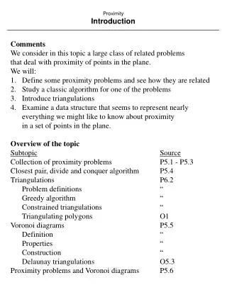
1. ProximityIntroduction Comments We consider in this topic a large class of related problems that deal with proximity of points in the plane. We will: 1. Define some proximity problems and see how they are related 2. Study a classic algorithm for one of the problems 3. Introduce triangulations 4. Examine a data structure that seems to represent nearly everything we might like to know about proximity in a set of points in the plane. Overview of the topic SubtopicSource Collection of proximity problems P5.1 - P5.3 Closest pair, divide and conquer algorithm P5.4 Triangulations P6.2 Problem definitions “ Greedy algorithm “ Constrained triangulations “ Triangulating polygons O1 Voronoi diagrams P5.5 Definition “ Properties “ Construction “ Delaunay triangulations O5.3 Proximity problems and Voronoi diagrams P5.6

2. ProximityProximity problems Closest pair CLOSEST PAIR INSTANCE: Set S = {p1, p2, ..., pN} of N points in the plane. QUESTION: Determine the two points of S whose mutual distance is smallest. Distance is defined as the usual Euclidean distance: distance(pi,pj) = sqrt((xi - xj)2 + (yi - yj)2). This problem is described as “one of the fundamental questions of computational geometry” in Preparata. Brute force A brute force solution is to compute the distance for every pair of points, saving the smallest; this requires O(dN2) time. The factor d is the number of dimensions, i.e., the number of coordinates involved in each distance computation. For d = 1, we can do better than O(N2), as follows: 1. Sort the N points (which are simply numbers). O(N log N) 2. Scan the sorted sequence (x1, x2, …, xN) computing xi+1 - xi for i = 1, 2, …, N-1. Save the smallest difference. This is optimal for d = 1. For d = 2, can we do better than O(2N2) O(N2)?

3. ProximityProximity problems All nearest neighbors ALL NEAREST NEIGHBORS INSTANCE: Set S = {p1, p2, ..., pN} of N points in the plane. QUESTION: Determine the “nearest neighbor” (point of minimum distance) for each point in S.

4. ProximityProximity problems Nearest neighbor relation, 1 “Nearest neighbor” is a relation on a set S as follows: point b is a nearest neighbor of point a, denoted ab, if distance(a,b) = min distance(a,c) cS - a (a, b, cS). The “nearest neighbor” relation is not symmetric, i.e., ab does not imply ba (though it could be true). Preparata, p. 186 says: “Note also that a point is not the nearest neighbor of a unique point (i.e., “” is not a function).” Perhaps slightly clearer: “Note that a point is not necessarily the nearest neighbor of a unique point, i.e., “” is not one-to-one, nor is it onto, as a point may have more than one nearest neighbor.”

5. ProximityProximity problems Nearest neighbor relation, 2 Footnote 2 on Preparata, p. 186: “Although a point can be the nearest neighbor of every other point, a point can have at most six nearest neighbors in two dimensions…” I think that is backwards, and should be: “Although a point can have every other point as a nearest neighbor, a point can be the nearest neighbor of at most six other points in two dimensions…” Point c has every other point as its nearest neighbor. c At most six points can have point c as their nearest neighbor.

6. ProximityProximity problems Euclidean minimum spanning tree EUCLIDEAN MINIMUM SPANNING TREE INSTANCE: Set S = {p1, p2, ..., pN} of N points in the plane. QUESTION: Construct a tree of minimum total length whose vertices are the points in S. A solution to this problem will be the N-1 pairs of points in S that comprise the edges of the tree. The (more general) Minimum Spanning Tree (MST) problem is usually formulated as a problem in graph theory: Given a graph G with N nodes and E weighted edges, find the subtree of G that includes every vertex with minimum total edge weight. In the Euclidean Minimum Spanning Tree (EMST) problem, the equivalent graph formulation has graph G complete (i.e., every pair of vertices is joined by an edge), with the edges weights just the distance between the vertices. Any algorithm that attacks EMST as a graph problem must necessarily take O(N2) time, because a MST on a graph must contain a shortest edge, and to find the shortest edge of the graph G, using a graph approach, requires examining N2 edges.) We seek a geometric algorithm for EMST that requires < O(N2) time.

7. ProximityProximity problems Triangulation TRIANGULATION INSTANCE: Set S = {p1, p2, ..., pN} of N points in the plane. QUESTION: Join the points in S with nonintersecting straight line segments so that every region internal to the convex hull of S is a triangle. A triangulation for a set S is not necessarily unique. As a planar graph, a triangulation on N vertices has  3N - 6 edges.

8. ProximityProximity problems Single-shot vs. search The previous problems (CLOSEST PAIR, ALL NEAREST NEIGHBORS, EUCLIDEAN MINIMUM SPANNING TREE, and TRIANGULATION) have been single shot. We now define two search-type proximity problems. Because these are search problems, repetitive mode is assumed, and thus preprocessing is allowed. Nearest neighbor search NEAREST NEIGHBOR SEARCH INSTANCE: Set S = {p1, p2, ..., pN} of N points in the plane. QUESTION: Given a query point q, which point pS is a nearest neighbor of q? p q

9. ProximityProximity problems k nearest neighbors k-NEAREST NEIGHBORS INSTANCE: Set S = {p1, p2, ..., pN} of N points in the plane. QUESTION: Given a query point q, determine the k points of S nearest to q. This problem is equivalent to the previous one for k = 1. The figure gives the solution for k = 3. q

10. ProximityProximity problems Element uniqueness Preparata defines a computational prototype as an archetypal problem, one which can act as a fundamental representative for a class of problems. For example, SATISFIABILITY for NP-complete problems, or SORTING from many problems in computational geometry. Another such problem is ELEMENT UNIQUENESS. ELEMENT UNIQUENESS INSTANCE: Set S = {x1, x2, ..., xN} of N real numbers. QUESTION: Are any two numbers xi, xj in S equal? It is shown in the text (Preparata, p. 192) using the algebraic decision tree model that a lower bound on time for ELEMENT UNIQUENESS is in (N log N). Three problems (SORTING, ELEMENT UNIQUENESS, and EXTREME POINTS (Preparata, p. 99)) all have lower bounds on time in (N log N). However, they are not easily transformable (“reducible”) to each other. Preparata asks: do they have a common “ancestor” problem that can be transformed into all of them? SORTING ? ELEMENT UNIQUENESS EXTREME POINTS O(N) O(N) O(N)

11. ProximityProximity problems Lower bounds The proximity problems we have defined can be transformed into each other as follows: ELEMENT CLOSEST ALL NEAREST UNIQUENESS PAIR NEIGHBORS (N log N) SORTING EUCLIDEAN MINIMUM (N log N) SPANNING TREE TRIANGULATION BINARY NEAREST NEIGHBOR SEARCH SEARCH (log N) k-NEAREST NEIGHBORS Here the arrow A B O((N)) means “transformable in time O((N)) in a way that proves the lower bound of B”. O(N) O(N) O(N) O(N) O(N) O(1) O(1)

12. ProximityProximity problems Search problems BINARY SEARCH O(1) NEAREST NEIGHBOR SEARCH BINARY SEARCH O(1)k-NEAREST NEIGHBORS Preparata defines BINARY SEARCH in a slightly unusual way, apparently to simplify the lower bounds proof. BINARY SEARCH INSTANCE: Set S = {x1, x2, ..., xN} of N real numbers and query real number q. Assume that for 1i, jN, i < jxi < xj (preprocessing). QUESTION (Usual): Find xi such that xiq < xi+1. QUESTION (Preparata): Find xi closest to q. xi-1 xi xi+1 Usual Preparata

13. ProximityProximity problems Search problems, 1 BINARY SEARCH has lower bound in (log N). Transform BINARY SEARCH to NEAREST NEIGHBOR SEARCH as follows: 1. Transform instance of BINARY SEARCH: S = {x1, x2, ..., xN} and q to an instance of NEAREST NEIGHBOR SEARCH: S = {(x1,0), (x2,0), ..., (xN,0)} and q = (q,0). O(N) time. 2. Solve NEAREST NEIGHBOR SEARCH for S and q; let (xi,0) be the solution. 3. Transform solution point (xi,0) to real number xi, which is the solution to BINARY SEARCH. O(1) time.  NEAREST NEIGHBOR has lower bound in (log N). Or does it?

14. ProximityProximity problems Search problems, 2 But, there seems to be a problem with this proof, as given in Preparata, p. 193: The O(N) transformation dominates the (log N) lower bound, voiding the result. We can get around that by considering the 1-dimensional version of NEAREST NEIGHBOR SEARCH, which has an instance identical to the instance of BINARY SEARCH. This resolution still has two difficulties: 1. It assumes that 2-dimensional NEAREST NEIGHBOR SEARCH has the same lower bound as the 1-dimensional version (this is probably easily proven). 2. However, the argument tantamount to a tautology, as 1-dimensional NEAREST NEIGHBOR SEARCH is the same problem as Preparata’s BINARY SEARCH. Can the proof be modified to start from the usual form of the BINARY SEARCH problem? We get a lower bound of (log N) for k-NEAREST NEIGHBORS directly by letting k = 1, in which case the problem is the same as NEAREST NEIGHBOR SEARCH, and thus gets a lower bound in (log N) by the same transformation.

15. ProximityProximity problems Closest pair ELEMENT UNIQUENESS has lower bound in (N log N). Transform ELEMENT UNIQUENESS to CLOSEST PAIR as follows: 1. Transform instance of ELEMENT UNIQUENESS: S = {x1, x2, ..., xN} to an instance of CLOSEST PAIR: S = {(x1,0), (x2,0), ..., (xN,0)}. O(N) time. 2. Solve CLOSEST PAIR for S; let (xi,0) and (xj,0) be the solution (the two closest points). 3. Transform this into a solution to ELEMENT UNIQUENESS: If xi = xj, return TRUE, else return FALSE. O(1) time.  CLOSEST PAIR has lower bound in (N log N).

16. ProximityProximity problems All nearest neighbors CLOSEST PAIR has lower bound in (N log N). Transform CLOSEST PAIR to ALL NEAREST NEIGHBORS as follows: 1. An instance of CLOSEST PAIR: S = {p1, p2, ..., pN} is an instance of ALL NEAREST NEIGHBORS: S = {p1, p2, ..., pN}. O(0) time. 2. Solve ALL NEAREST NEIGHBORS for S; let A = {(p1,q1), (p2,q2), …, (pN,qN)} be the solution (qiS, a nearest neighbor for each point in S). 3. Transform this into a solution to CLOSEST PAIR: For each pair (pj,qi) A, compute distance(pj,qi). Save the smallest. O(N) time. ALL NEAREST NEIGHBORS has lower bound in (N log N).

17. ProximityProximity problems Euclidean minimum spanning tree SORTING has lower bound in (N log N). Transform SORTING to EUCLIDEAN MINIMUM SPANNING TREE (EMST) as follows: 1. An instance of SORTING: S = {x1, x2, ..., xN} to an instance of EMST: S = {(x1,0), (x2,0), ..., (xN,0)}. O(N) time. 2. Solve EMST for S. A set of points along the x axis has a unique EMST, where there is an edge ((xi,0),(xj,0)) iff xi and xj are consecutive in sorted order. Let T = {(xi1,xj1), (xi2,xj2), …, (xiN,xjN)} be the solution (the edges of the EMST, in no particular order). 3. Transform this into a solution to SORTING: Initialize an array A of N entries: A.first = TRUE, A.next = 0. For each edge (xi1,xj1) in T: A.next[i1] = j1, A.first[j1] = FALSE. Scan A to find A.first = TRUE. From there, follow the A.next indices to read off the sorted order. O(N) time. EMST has lower bound in (N log N). Step 3 is not given in Preparata, it is simply described as “a simple exercise”.

18. ProximityProximity problems Triangulation SORTING has lower bound in (N log N). Transform SORTING to TRIANGULATION as follows: 1. An instance of SORTING: S = {x1, x2, ..., xN} to an instance of TRIANGULATION: S = {(x1,0), (x2,0), ..., (xN,0)}  {(0,-1)}. O(N) time. 2. Solve TRIANGULATION for S. Set of points S has a unique triangulation, shown in the figure. Let T = {(xi1,xj1), (xi2,xj2), …, (xiN,xjN)} be the solution (the edges of the triangulation, in no particular order). 3. Transform this into a solution to SORTING in a manner similar to the procedure for EMST, ignoring edges that include point (0,-1). O(N) time. TRIANGULATION has lower bound in (N log N).