Download
1 / 25
250 likes | 369 Views
This tutorial provides a comprehensive guide for analyzing gamma-ray emissions from the Sun, specifically focusing on the quiet Sun period. It utilizes the Fermi-LAT data to explore inverse Compton scattering and interactions of Galactic cosmic rays with the solar atmosphere. The package includes tools like XSPEC for modeling and software for likelihood analysis. Users will find detailed instructions for data extraction, background evaluation, and model fitting essentials for sophisticated astrophysical research. The Sun's gamma-ray flux variations in relation to solar activity are also explored.

E N D
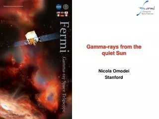
Gamma-rays from the quiet Sun Nicola Omodei Stanford
SolarTutorial • Get the needed files: • https://www.dropbox.com/sh/s8io1bq5yvk966j/3F6Rq3xTI4 • Unpack the SolarTutorial_src.tgz and SolarTutorial_data.tgz file into the tools directory. • tools/SolarTutorial should look like: • XSPEC/ (models for XSPEC) • lleBackground/ (tool for extracting the LLE background) • src/ (python code) • data/ (data, FT1, FT2 and LLE, template file for likelihood analysis, isotropic model and galactic diffuse model)
γ p Quite Sun gamma-ray emission Sun is bright in gammas due to interactions of Galactic cosmic rays (CR) • Inverse Compton (IC) emission from the Sun • idea and theory: Moskalenko et al. 2006, Orlando & Strong 2007, 2008 e- e- η < radial e- > p γ < Galactic CRs + 2) Solar disk emission due to interactions of CR particles with solar atmosphere model : Seckel 91, upper-limit detection: Thompson 97 First detection (EGRET): Orlando & Strong, 2008 FERMI/LAT: high statistical significance for a clear separation of the components! 2011ApJ...734..116A
Solar Activity (SA) and Cosmic rays (CR) Solar gamma-ray flux depends on CRs flux Max SA -> min CR flux Min SA -> max CR flux • - SA was in its minimum during the period analyzed in the Fermi LAT paper • SA is now increasing and expected to peak around 2013
Fermi paper: LAT data selection • 18 months data • Analysis in Sun-centered system • Zenith angle < 105° (to avoid the Earth’s emission) • Galactic Plane Cut (|b|>30°) (to reduce the background) • Moon-Sun angular separation >40° • Avoided the brightest sources, F(>100 MeV) above 2e-7 cm-2s-1 • Only a small percentage of the data survives Counts map >100 MeV 7
Ephemerides in a nutshell #!/usr/bin/env python import pyLikelihood as pl import os from math import * def d(x): return degrees(x) def r(x): return radians(x) def getJD(met): if met > 252460801: met-=1 # 2008 leap second if met > 157766400: met-=1 # 2005 leap second if met > 362793601: met-=1 # 2012 leap second return (pl.JulianDate.seconds(pl.JulianDate_missionStart())+met)/pl.JulianDate.secondsPerDay def _jd_from_met(met): jd = pl.JulianDate(getJD(met)) return jd def getSunPosition( met ): os.environ['TIMING_DIR']=os.path.join(os.environ['HEADAS'],"refdata") sun=pl.SolarSystem(pl.SolarSystem.SUN) return sun.direction(_jd_from_met(met)) def rotation(x,y,p): xr=r(x) yr=r(y) pr=r(p) x1= d(atan2(sin(xr)*cos(pr) + tan(yr)*sin(pr), cos(xr))) y1 = d(asin(sin(yr)*cos(pr) - cos(yr)*sin(xr)*sin(pr))) return x1,y1 def equatorial2ecliptic(ra,dec): EPS = 23.439292 # THIS IS THE OBMIQUITY AS J2000 (lon,lat)=rotation(ra,dec,EPS) if lon<0: lon+=360 return (lon,lat) ./sunpos.py 376358403.0 Difference from USNO position: 0.0007530°
Sun Centered coordinates • At each instant, the rotation brings • RA,DEC -> ecliptic lon-Sun lon, ecliptic latitude. • The idea is to replace the RA,DEC with the new coordinates: • FT1 file (RA,DEC) • FT2 file: (RA_ZENITH, DEC_ZENITH), (RA_SCZ,DEC_SCZ),(RA_SCX, DEC_SCX) ./suncenter.py –ft1 ft1fileName ./suncenter.py –ft2 ft2fileName
Background determination • Galactic and extragalactic emission along the ecliptic • 2 methods for evaluating the background: • Based on data • Based on simulations
Based on data:Fake source method • A fake source follows the path of the real source but many degrees away (integrated along the ecliptic)
Photon density profile >100 MeV Sun Fake-Sun background
Angular profiles: evidence of extended emission • Sun Data • BKG • IC • Disk + Bkg+IC > 500 MEV Good description of the background Zoom in Angular distribution well fitted by both disk and IC components. 13
Disk SED s.i.=-2 SED for the disk emission compared with model predictions.
Analysis method • Model “Independent” Fit for the IC Component • IC-ring models with Pls (RINGS: 5-11-20°) • Model for Disk point-like Component • Point source modeled with a PL2 • Model for background Component • spatially uniform nested rings, (RINGS 10-14-17.3-20°) spectrum from fake sun
IC: Results IC flux IC differential spectrum
Disk results Energy
Including the quite sun in Solar flare analysis <source name=”SunDisk" type="PointSource"> <!-- point source units are cm^-2 s^-1 MeV^-1 --> <spectrum type="PowerLaw2"> <parameter free=”0" max="1000.0" min="1e-05" name="Integral" scale="1e-06" value=”0.463"/> <parameter free=”0" max="-1.0" min="-5.0" name="Index" scale="1.0" value="-2.11"/> <parameter free="0" max="200000.0" min="20.0" name="LowerLimit" scale="1.0" value="20.0"/> <parameter free="0" max="200000.0" min="20.0" name="UpperLimit" scale="1.0" value="2e5"/> </spectrum> <spatialModel type="SkyDirFunction"> <parameter free="0" max="360." min="-360." name="RA" scale="1.0" value=”0"/> <parameter free="0" max="90." min="-90." name="DEC" scale="1.0" value=”0"/> </spatialModel> </source> This is for Sun Center coordinates, otherwise replace with R.A. and Dec. of the Sun • The Sun is a faint source of gamma-rays, not detected on hour long time scale. • Depending on its position, can be detected in few days.
Take at home • Calculate the position of the Sun (sunpos.py) • Calculate the sun-centered FT1 and FT2 (suncenter.py) • For long duration flares > 6 hr you will need to work in sun centered coordinates.
SolarTutorial • Get the needed files: • https://www.dropbox.com/sh/s8io1bq5yvk966j/3F6Rq3xTI4 • Unpack the SolarTutorial_src.tgz and SolarTutorial_data.tgz file into the tools directory. • tools/SolarTutorial should look like: • XSPEC/ (models for XSPEC) • lleBackground/ (tool for extracting the LLE background) • src/ (python code) • data/ (data, FT1, FT2 and LLE, template file for likelihood analysis, isotropic model and galactic diffuse model)
What’s in there • ProgressBar.py* (helper function to display a progress bar…) • SFLARE110307_analysis.py* (executable, run the analysis in different TIME bins, in equatorial coordinates) • SFLARE110307_analysis_SC.py* (executable run the analysis in 1 time bin, in sun-centered coordinates) • analysis.py (this is the script containing the analysis steps) • makeProfileLikelihood.py* (Used to draw a profile likelihood, once the analysis is finished) • myscripts.py (wrapper around ST) • plotSED.py* (plot the SED) • setup.sh (you can use to setup your environment (ignore for now) • suncenter.py* (compute the sun center ft1 and ft2 files) • sunpos.py* (compute the position of the sun) • xspec_cmd.tcl (example of xspec command)
Inverse Compton models • Uncertainty in the solar modulation of electrons close to the Sun • Force field approximation for e- spectrum modulation (Gleeson & Axford 68) • Starting from the Fermi electron spectrum at 1AU, 3 MODELS with Φ0(1AU)=400MV, but different formulations of Φ(r): MODEL 1 and MODEL 2 assume additional modulation <1AU, MODEL 3 assumes the e- spectrum constant <1AU. E- spectrum at r=1AU as measured by Fermi Modulation potential LIS
Electron spectra for IC models LIS galprop AMS 02 Fermi LIS 1AU At 0.3AU MODEL3 e- constant <1AU MODEL1 (400MV) MODEL2 (400MV)
Quiet Solar emission: pion decay • Solar disk emission due to interactions of CR particles with solar atmosphere Seckel ‘91 NAIVE: no B Mirrored showers, reflected by B back to the surface NOMINAL: includes CR diffusion Cascade developpement in forward direction F(> 100MeV) = (0.22−0.65) 10−7 cm-2 s-1 for nominal